Deep Learning 1_深度学习UFLDL教程：Sparse Autoencoder练习（斯坦福大学深度学习教程）

1前言

本人写技术博客的目的，其实是感觉好多东西，很长一段时间不动就会忘记了，为了加深学习记忆以及方便以后可能忘记后能很快回忆起自己曾经学过的东西。

首先，在网上找了一些资料，看见介绍说UFLDL很不错，很适合从基础开始学习，Adrew Ng大牛写得一点都不装B，感觉非常好，另外对我们英语不好的人来说非常感谢，此教程的那些翻译者们！如余凯等。因为我先看了一些深度学习的文章，但是感觉理解得不够，一般要自己编程或者至少要看懂别人的程序才能理解深刻，所以我根据该教程的练习，一步一步做起，当然我也参考了一些别人已编好的程序，这是为了节省时间，提高效率，还可以学习其他人好的编程习惯。

另外感觉tornadomeet比较牛，写的博客非常细，适合我这种初学者学习，在此非常感谢！我也关注了他的微博，现在他在网易还在从事深度学习。

此练习是按UFLDL的Sparse Autoencoder练习来的做的。

2练习基础

看本文练习请先看其教程第一节，里面有它的原理及相关符号约定。

注意：本文的程序已经是矢量化编程的结果，所以即使是检查梯度也比较快。

以下基础是引用自tornadomeet的博客，感觉写的很好，一看就知道他非常详细地读了Ng提供的每个程序。但是我也加了自己的一些东西。

　　一些malab函数：

　　bsxfun:

　　C=bsxfun(fun,A,B)表达的是两个数组A和B间元素的二值操作，fun是函数句柄或者m文件，或者是内嵌的函数。在实际使用过程中fun有很多选择比如说加，减等，前面需要使用符号’@’.一般情况下A和B需要尺寸大小相同，如果不相同的话，则只能有一个维度不同，同时A和B中在该维度处必须有一个的维度为1。比如说bsxfun(@minus, A, mean(A))，其中A和mean(A)的大小是不同的，这里的意思需要先将mean(A)扩充到和A大小相同，然后用A的每个元素减去扩充后的mean(A)对应元素的值。

　　rand：

　　生成均匀分布的伪随机数。分布在（0~1）之间
　　主要语法：rand(m,n)生成m行n列的均匀分布的伪随机数
             rand(m,n,'double')生成指定精度的均匀分布的伪随机数，参数还可以是'single'
             rand(RandStream,m,n)利用指定的RandStream(我理解为随机种子)生成伪随机数

　　randn：

　　生成标准正态分布的伪随机数（均值为0，方差为1）。主要语法：和上面一样

　　randi：

　　生成均匀分布的伪随机整数 
 　 主要语法：randi（iMax）在闭区间（0，iMax）生成均匀分布的伪随机整数 
             randi（iMax，m，n）在闭区间（0，iMax）生成mXn型随机矩阵
             r = randi([iMin,iMax],m,n)在闭区间（iMin，iMax）生成mXn型随机矩阵

　　exist:

　　测试参数是否存在，比如说exist('opt_normalize', 'var')表示检测变量opt_normalize是否存在，其中的’var’表示变量的意思。

　　colormap:

　　设置当前常见的颜色值表。

　　floor：

　　floor(A):取不大于A的最大整数。

　　ceil:

　　ceil(A):取不小于A的最小整数。

　　imagesc:

　　imagesc和image类似，可以用于显示图像。比如imagesc(array,'EraseMode','none',[-1 1])，这里的意思是将array中的数据线性映射到[-1,1]之间，然后使用当前设置的颜色表进行显示。此时的[-1,1]充满了整个颜色表。背景擦除模式设置为node，表示不擦除背景。

　　repmat:

　　该函数是扩展一个矩阵并把原来矩阵中的数据复制进去。比如说B = repmat(A,m,n)，就是创建一个矩阵B，B中复制了共m*n个A矩阵，因此B矩阵的大小为[size(A,1)*m  size(A,2)*m]。

matlab中的@用法：

问：f=@(x)acos(x)表示什么意思？其中@代表什么？
答：表示f为函数句柄，@是定义句柄的运算符。f=@(x)acos(x) 相当于建立了一个函数文件：
% f.m
function  y=f(x)
y=acos(x);

若有下列语句：xsqual=@(x)1/2.*(x==-1/2)+1.*(x>-1/28&x<1/2)+1.2.*(x==-1/2);

则相当于建立了一个函数文件：

% xsqual.m

function y=xsqual(x)

y=1/2.*(x==-1/2)+1.*(x>-1/28&x<1/2)+1.2.*(x==-1/2);

函数句柄的好处
       ①提高运行速度。因为matlab对函数的调用每次都是要搜索所有的路径，从set path中我们可以看到，路径是非常的多的，所以如果一个函数在你的程序中需要经常用到的话，使用函数句柄，对你的速度会有提高的。
       ②使用可以与变量一样方便。比如说，我再这个目录运行后，创建了本目录的一个函数句柄，当我转到其他的目录下的时候，创建的函数句柄还是可以直接调用的，而不需要把那个函数文件拷贝过来。因为你创建的function handles中，已经包含了路径，

　　使用函数句柄的作用：

　　不使用函数句柄的情况下，对函数多次调用，每次都要为该函数进行全面的路径搜索，直接影响计算速度，借助句柄可以完全避免这种时间损耗。也就是直接指定了函数的指针。函数句柄就像一个函数的名字，有点类似于C++程序中的引用。

代价函数  为：

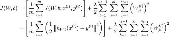
，其中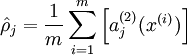   

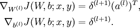
计算梯度需要用到的公式：

对输出层（第  层），计算：

    其中，y是希望输出得到数据，即：y=x

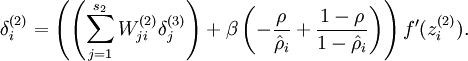  其中，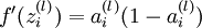 

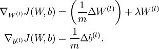
令  , 

3练习步骤

1.产生训练集。从10张512*512的图片中，随机选择10000张8*8的小图块，然后再把它归一化，得到训练集patches。具体见程序 sampleIMAGES.m

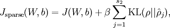
2.计算出代价函数 J_sparse(W,b) 及其梯度。具体见程序sparseAutoencoderCost.m。

3.通过函数 computeNumericalGradient.m计算出大概梯度（EPSILON = 10^-4），然后通过函数checkNumericalGradient.m检查上一步写的计算梯度的代码是否正确。首先，通过计算函数 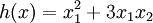在点[4，10]处的梯度对比用computeNumericalGradient.m中的方法计算该函数的梯度，这两者梯度的差值小于10^-9就代表computeNumericalGradient.m中方法是正确的。然后，用computeNumericalGradient.m中方法计算代价函数 J_sparse(W,b) 的梯度对比用sparseAutoencoderCost.m中的方法计算代价函数 J_sparse(W,b) 的梯度，如果这两者梯度的差值小于10^-9就证明sparseAutoencoderCost.m中方法是正确的。

4.训练稀疏自动编码器。用的 L-BFGS算法（注意：这个算法不能将它用于商业用途，若用与商业用途的话，可以使用fminlbfgs函数，他比L-BFGS慢但可用于商业用途），具体见文件夹 minFunc。另外，初始化参数矩阵θ（包含W⁽¹⁾,W⁽²⁾,b⁽¹⁾,b⁽²⁾）时，W⁽¹⁾,W^{(2)的初始值是从 中随机均匀分布产生，其中 n_{in是隐藏层神经元个数， nout 是输出层神经元个数。b(1),b(2)初始化为0.}}

5.可视化结果。点击train.m运行总程序，训练稀疏自动编码器，得到可视化结果。把产生的权重结果可视化，通过它我们能够知道，该算法究竟从图片中学习了哪些特征。

运行整个程序，从开始产生训练集到最后得到可视化结果，所用的时间为144.498443 seconds。

具体显示第一层特征的可视化函数display_network.m的详细注释可见：Deep Learning八：Stacked Autocoders and Implement deep networks for digit classification_Exercise（斯坦福大学深度学习教程UFLDL）

运行结果为：

训练集为：

特征可视化结果为：

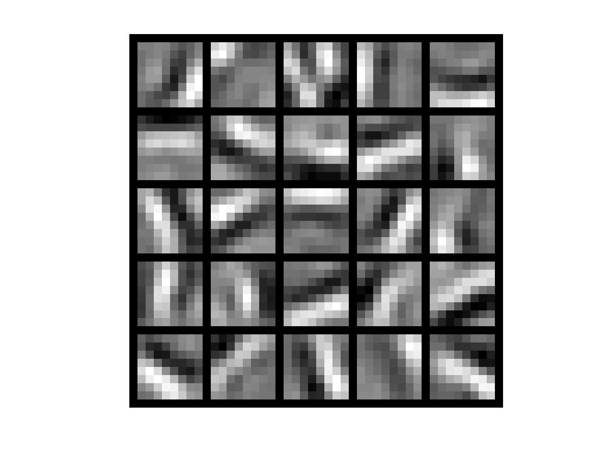
可以看出，稀疏自动编码器学习到的特征实际上是图像的边缘

>> train
Elapsed time is 0.034801 seconds.
38.0000 38.0000
12.0000 12.0000

The above two columns you get should be very similar.
(Left-Your Numerical Gradient, Right-Analytical Gradient)

2.1452e-12

上面是通过计算函数 在点[4，10]处的梯度对比用computeNumericalGradient.m中的方法计算该函数的梯度，这两者梯度的差值，可见他小于10^-9

7.8813e-11

Iteration FunEvals Step Length Function Val Opt Cond
1 4 7.66801e-02 8.26267e+00 2.99521e+02
2 5 1.00000e+00 4.00448e+00 1.59279e+02

上面是用computeNumericalGradient.m中方法计算代价函数 J_sparse(W,b) 的梯度对比用sparseAutoencoderCost.m中的方法计算代价函数 J_sparse(W,b) 的梯度，可见这两者梯度的差值小于10^-9

4代码及注释

train.m

%% CS294A/CS294W Programming Assignment Starter Code

% Instructions
% ------------
%
% This file contains code that helps you get started on the
% programming assignment. You will need to complete the code in sampleIMAGES.m,
% sparseAutoencoderCost.m and computeNumericalGradient.m.
% For the purpose of completing the assignment, you do not need to
% change the code in this file.
%
%%======================================================================
%% STEP 0: Here we provide the relevant parameters values that will
% allow your sparse autoencoder to get good filters; you do not need to
% change the parameters below.第0步：提供可得到较好滤波器的相关参数值，不得改变以下参数

visibleSize = 8*8; % number of input units 输入层单元数
hiddenSize = 25; % number of hidden units隐藏层单元数
sparsityParam = 0.01; % desired average activation of the hidden units.稀疏值
% (This was denoted by the Greek alphabet rho, which looks like a lower-case "p",
% in the lecture notes).
lambda = 0.0001; % weight decay parameter 权重衰减系数
beta = 3; % weight of sparsity penalty term稀疏值惩罚项的权重

%%======================================================================
%% STEP 1: Implement sampleIMAGES 第1步：实现图片采样
%
% 实现图片采样后，函数display_network从训练集中随机显示200张
% After implementing sampleIMAGES, the display_network command should
% display a random sample of 200 patches from the dataset

patches = sampleIMAGES;
display_network(patches(:,randi(size(patches,2),200,1)),8);%从10000张中随机选择200张显示

% Obtain random parameters theta初始化参数向量theta
theta = initializeParameters(hiddenSize, visibleSize);

%%======================================================================
%% STEP 2: Implement sparseAutoencoderCost
%
% 在计算代价函数时，可以一次计算其所有的元素项值（均方差项、权重衰减项、惩罚项），但是一步一步地计算各元素项值，
% 然后每步完成后运行梯度检验的方法可能会更容易实现，建议按照下面的步骤来实现函数sparseAutoencoderCost：
% You can implement all of the components (squared error cost, weight decay term,
% sparsity penalty) in the cost function at once, but it may be easier to do
% it step-by-step and run gradient checking (see STEP 3) after each step. We
% suggest implementing the sparseAutoencoderCost function using the following steps:
%
% (a) Implement forward propagation in your neural network, and implement the
% squared error term of the cost function. Implement backpropagation to
% compute the derivatives. Then (using lambda=beta=0), run Gradient Checking
% to verify that the calculations corresponding to the squared error cost
% term are correct.实现神经网络中的前向传播和代价函数中的均方差项。通过反向传导计算偏导数。
% 然后运行梯度检验法来检查均方差项是否计算错误。
%
% (b) Add in the weight decay term (in both the cost function and the derivative
% calculations), then re-run Gradient Checking to verify correctness.在代价函数和偏导数计算中
% 加入权重衰减项，然后运行梯度检验法来检查其正确性。
%
% (c) Add in the sparsity penalty term, then re-run Gradient Checking to
% verify correctness.加入惩罚项，然后运行梯度检验法来检查其正确性。
%
% Feel free to change the training settings when debugging your
% code. (For example, reducing the training set size or
% number of hidden units may make your code run faster; and setting beta
% and/or lambda to zero may be helpful for debugging.) However, in your
% final submission of the visualized weights, please use parameters we
% gave in Step 0 above.

[cost, grad] = sparseAutoencoderCost(theta, visibleSize, hiddenSize, lambda, ...
sparsityParam, beta, patches);

%%======================================================================
%% STEP 3: Gradient Checking
%
% Hint: If you are debugging your code, performing gradient checking on smaller models
% and smaller training sets (e.g., using only 10 training examples and 1-2 hidden
% units) may speed things up.

% First, lets make sure your numerical gradient computation is correct for a
% simple function. After you have implemented computeNumericalGradient.m,
% run the following:
checkNumericalGradient();

% Now we can use it to check your cost function and derivative calculations
% for the sparse autoencoder.
numgrad = computeNumericalGradient( @(x) sparseAutoencoderCost(x, visibleSize, ...
hiddenSize, lambda, ...
sparsityParam, beta, ...
patches), theta);

% Use this to visually compare the gradients side by side
disp([numgrad grad]);

% Compare numerically computed gradients with the ones obtained from backpropagation
diff = norm(numgrad-grad)/norm(numgrad+grad);
disp(diff); % Should be small. In our implementation, these values are
% usually less than 1e-9.

% When you got this working, Congratulations!!!

%%======================================================================
%% STEP 4: After verifying that your implementation of
% sparseAutoencoderCost is correct, You can start training your sparse
% autoencoder with minFunc (L-BFGS).

% Randomly initialize the parameters
theta = initializeParameters(hiddenSize, visibleSize);

% Use minFunc to minimize the function
addpath minFunc/
options.Method = 'lbfgs'; % Here, we use L-BFGS to optimize our cost
% function. Generally, for minFunc to work, you
% need a function pointer with two outputs: the
% function value and the gradient. In our problem,
% sparseAutoencoderCost.m satisfies this.
options.maxIter = 400;	 % Maximum number of iterations of L-BFGS to run
options.display = 'on';

[opttheta, cost] = minFunc( @(p) sparseAutoencoderCost(p, ...
visibleSize, hiddenSize, ...
lambda, sparsityParam, ...
beta, patches), ...
theta, options);

%%======================================================================
%% STEP 5: Visualization

W1 = reshape(opttheta(1:hiddenSize*visibleSize), hiddenSize, visibleSize);
display_network(W1', 12);

print -djpeg weights.jpg % save the visualization to a file

　　

sampleIMAGES.m

function patches = sampleIMAGES()
% sampleIMAGES
% Returns 10000 patches for training

load IMAGES;    % load images from disk 

patchsize = 8;  % we'll use 8x8 patches
numpatches = 10000;

% Initialize patches with zeros.  Your code will fill in this matrix--one
% column per patch, 10000 columns.
patches = zeros(patchsize*patchsize, numpatches);

%% ---------- YOUR CODE HERE --------------------------------------
%  Instructions: Fill in the variable called "patches" using data
%  from IMAGES.
%
%  IMAGES is a 3D array containing 10 images
%  For instance, IMAGES(:,:,6) is a 512x512 array containing the 6th image,
%  and you can type "imagesc(IMAGES(:,:,6)), colormap gray;" to visualize
%  it. (The contrast on these images look a bit off because they have
%  been preprocessed using using "whitening."  See the lecture notes for
%  more details.) As a second example, IMAGES(21:30,21:30,1) is an image
%  patch corresponding to the pixels in the block (21,21) to (30,30) of
%  Image 1
tic
image_size=size(IMAGES);
i=randi(image_size(1)-patchsize+1,1,numpatches);%生成元素值随机为大于0且小于image_size(1)-patchsize+1的1行numpatches矩阵
j=randi(image_size(2)-patchsize+1,1,numpatches);
k=randi(image_size(3),1,numpatches);
for num=1:numpatches
        patches(:,num)=reshape(IMAGES(i(num):i(num)+patchsize-1,j(num):j(num)+patchsize-1,k(num)),1,patchsize*patchsize);
end
toc

%% ---------------------------------------------------------------
% For the autoencoder to work well we need to normalize the data
% Specifically, since the output of the network is bounded between [0,1]
% (due to the sigmoid activation function), we have to make sure
% the range of pixel values is also bounded between [0,1]
patches = normalizeData(patches);

end

%% ---------------------------------------------------------------
function patches = normalizeData(patches)

% Squash data to [0.1, 0.9] since we use sigmoid as the activation
% function in the output layer

% Remove DC (mean of images). 把patches数组中的每个元素值都减去mean(patches)
patches = bsxfun(@minus, patches, mean(patches));

% Truncate to +/-3 standard deviations and scale to -1 to 1
pstd = 3 * std(patches(:));%把patches的标准差变为其原来的3倍
patches = max(min(patches, pstd), -pstd) / pstd;%因为根据3sigma法则，95%以上的数据都在该区域内
                                                % 这里转换后将数据变到了-1到1之间
% Rescale from [-1,1] to [0.1,0.9]
patches = (patches + 1) * 0.4 + 0.1;

end

　　sparseAutoencoderCost.m

function [cost,grad] = sparseAutoencoderCost(theta, visibleSize, hiddenSize, ...
                                             lambda, sparsityParam, beta, data)

% visibleSize:输入层神经单元节点数 the number of input units (probably 64)
% hiddenSize:隐藏层神经单元节点数 the number of hidden units (probably 25)
% lambda: 权重衰减系数weight decay parameter
% sparsityParam: 稀疏性参数The desired average activation for the hidden units (denoted in the lecture
%                           notes by the greek alphabet rho, which looks like a lower-case "p").
% beta: 稀疏惩罚项的权重weight of sparsity penalty term
% data: 训练集Our 64x10000 matrix containing the training data.  So, data(:,i) is the i-th training example.
% theta：参数向量，包含W1、W2、b1、b2

% The input theta is a vector (because minFunc expects the parameters to be a vector).
% We first convert theta to the (W1, W2, b1, b2) matrix/vector format, so that this
% follows the notation convention of the lecture notes. 

W1 = reshape(theta(1:hiddenSize*visibleSize), hiddenSize, visibleSize);
W2 = reshape(theta(hiddenSize*visibleSize+1:2*hiddenSize*visibleSize), visibleSize, hiddenSize);
b1 = theta(2*hiddenSize*visibleSize+1:2*hiddenSize*visibleSize+hiddenSize);
b2 = theta(2*hiddenSize*visibleSize+hiddenSize+1:end);

% Cost and gradient variables (your code needs to compute these values).
% Here, we initialize them to zeros.
cost = 0;
W1grad = zeros(size(W1));
W2grad = zeros(size(W2));
b1grad = zeros(size(b1));
b2grad = zeros(size(b2));

%% ---------- YOUR CODE HERE --------------------------------------
%  Instructions: Compute the cost/optimization objective J_sparse(W,b) for the Sparse Autoencoder,
%                and the corresponding gradients W1grad, W2grad, b1grad, b2grad.
%
% W1grad, W2grad, b1grad and b2grad should be computed using backpropagation.
% Note that W1grad has the same dimensions as W1, b1grad has the same dimensions
% as b1, etc.  Your code should set W1grad to be the partial derivative of J_sparse(W,b) with
% respect to W1.  I.e., W1grad(i,j) should be the partial derivative of J_sparse(W,b)
% with respect to the input parameter W1(i,j).  Thus, W1grad should be equal to the term
% [(1/m) \Delta W^{(1)} + \lambda W^{(1)}] in the last block of pseudo-code in Section 2.2
% of the lecture notes (and similarly for W2grad, b1grad, b2grad).
%
% Stated differently, if we were using batch gradient descent to optimize the parameters,
% the gradient descent update to W1 would be W1 := W1 - alpha * W1grad, and similarly for W2, b1, b2.
%
%1.前向传播forward propagation
data_size=size(data);
active_value2=repmat(b1,1,data_size(2));
active_value3=repmat(b2,1,data_size(2));
active_value2=sigmoid(W1*data+active_value2);                %第2层激活值
active_value3=sigmoid(W2*active_value2+active_value3);       %第3层激活值
%2.计算代价函数computing error term and cost
ave_square=sum(sum((active_value3-data).^2)./2)/data_size(2);%均方差项
weight_decay=lambda/2*(sum(sum(W1.^2))+sum(sum(W2.^2)));     %权重衰减项

p_real=sum(active_value2,2)./data_size(2); %对active_value2每行求和，再平均，得到每个隐藏单元的平均活跃度（25行1列）
p_para=repmat(sparsityParam,hiddenSize,1); %稀疏性参数（25行1列）
sparsity=beta.*sum(p_para.*log(p_para./p_real)+(1-p_para).*log((1-p_para)./(1-p_real)));%惩罚项
cost=ave_square+weight_decay+sparsity;     %代价函数

delta3=(active_value3-data).*(active_value3).*(1-active_value3); %第3层残差
average_sparsity=repmat(sum(active_value2,2)./data_size(2),1,data_size(2));%每个隐藏单元的平均活跃度（25行10000列）
default_sparsity=repmat(sparsityParam,hiddenSize,data_size(2));  %稀疏性参数（25行10000列）
sparsity_penalty=beta.*(-(default_sparsity./average_sparsity)+((1-default_sparsity)./(1-average_sparsity)));
delta2=(W2'*delta3+sparsity_penalty).*((active_value2).*(1-active_value2));%第2层残差
%3.反向传导backword propagation
W2grad=delta3*active_value2'./data_size(2)+lambda.*W2;  %W2梯度
W1grad=delta2*data'./data_size(2)+lambda.*W1;           %W1梯度
b2grad=sum(delta3,2)./data_size(2);                     %b2梯度
b1grad=sum(delta2,2)./data_size(2);                     %b1梯度

%-------------------------------------------------------------------
% After computing the cost and gradient, we will convert the gradients back
% to a vector format (suitable for minFunc).  Specifically, we will unroll
% your gradient matrices into a vector.

grad = [W1grad(:) ; W2grad(:) ; b1grad(:) ; b2grad(:)];

end

%-------------------------------------------------------------------
% Here's an implementation of the sigmoid function, which you may find useful
% in your computation of the costs and the gradients.  This inputs a (row or
% column) vector (say (z1, z2, z3)) and returns (f(z1), f(z2), f(z3)). 

function sigm = sigmoid(x)

    sigm = 1 ./ (1 + exp(-x));
end

　　computeNumericalGradient.m 

function numgrad = computeNumericalGradient(J, theta)
% numgrad = computeNumericalGradient(J, theta)
% theta: 参数向量，包含W1、W2、b1、b2；a vector of parameters
% J: a function that outputs a real-number. Calling y = J(theta) will return the
% function value at theta. 

% Initialize numgrad with zeros
numgrad = zeros(size(theta));

%% ---------- YOUR CODE HERE --------------------------------------
% Instructions:
% Implement numerical gradient checking, and return the result in numgrad.
% (See Section 2.3 of the lecture notes.)
% You should write code so that numgrad(i) is (the numerical approximation to) the
% partial derivative of J with respect to the i-th input argument, evaluated at theta.
% I.e., numgrad(i) should be the (approximately) the partial derivative of J with
% respect to theta(i).
%
% Hint: You will probably want to compute the elements of numgrad one at a time.
EPSILON=0.0001;
for i=1:size(theta)
    theta_plus=theta;
    theta_minu=theta;
    theta_plus(i)=theta_plus(i)+EPSILON;
    theta_minu(i)=theta_minu(i)-EPSILON;
    numgrad(i)=(J(theta_plus)-J(theta_minu))/(2*EPSILON);
end

%% ---------------------------------------------------------------
end

另外，checkNumericalGradient.m、display_network.m、minFunc、initializeParameters.m函数见UFLDL的 sparseae_exercise.zip。

参考资料：

Exercise:Sparse Autoencoder

http://www.cnblogs.com/hrlnw/archive/2013/06/08/3127162.html

http://www.cnblogs.com/tornadomeet/archive/2013/03/20/2970724.html

http://www.cnblogs.com/cj695/p/4498699.html