(原创)（三）机器学习笔记之Scikit Learn的线性回归模型初探

一、Scikit Learn中使用estimator三部曲

1. 构造estimator

2. 训练模型：fit

3. 利用模型进行预测：predict

二、模型评价

模型训练好后，度量模型拟合效果的常见准则有：

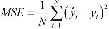
1.      均方误差（mean squared error，MSE）：

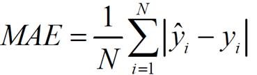
2.      平均绝对误差（mean absolute error，MAE）

3.      R2 score：scikit learn线性回归模型的缺省评价准则，既考虑了预测值与真值之间的差异，也考虑了问题本身真值之间的差异：

4.      检测残差的分布

检测残差是否是均值为0的正态分布。

三、Scikit Learn中的线性回归

1. 线性回归，梯度下降法模型优化参数

sklearn.linear_model.LinearRegression(fit_intercept=True, normalize=False, copy_X=True, n_jobs=1)

参数：

Ordinary least squares Linear Regression.

Parameters:

fit_intercept : boolean, optional whether to calculate the intercept for this model. If set to false, no intercept will be used in calculations (e.g. data is expected to be already centered). normalize : boolean, optional, default False If True, the regressors X will be normalized before regression. This parameter is ignored when fit_intercept is set to False. When the regressors are normalized, note that this makes the hyperparameters learnt more robust and almost independent of the number of samples. The same property is not valid for standardized data. However, if you wish to standardize, please use preprocessing.StandardScaler before calling fit on an estimator with normalize=False. copy_X : boolean, optional, default True If True, X will be copied; else, it may be overwritten. n_jobs : int, optional, default 1 The number of jobs to use for the computation. If -1 all CPUs are used. This will only provide speedup for n_targets > 1 and sufficient large problems.

Attributes:

coef_ : array, shape (n_features, ) or (n_targets, n_features) Estimated coefficients for the linear regression problem. If multiple targets are passed during the fit (y 2D), this is a 2D array of shape (n_targets, n_features), while if only one target is passed, this is a 1D array of length n_features. residues_ : array, shape (n_targets,) or (1,) or empty Sum of residuals. Squared Euclidean 2-norm for each target passed during the fit. If the linear regression problem is under-determined (the number of linearly independent rows of the training matrix is less than its number of linearly independent columns), this is an empty array. If the target vector passed during the fit is 1-dimensional, this is a (1,) shape array. New in version 0.18. intercept_ : array Independent term in the linear model.

训练：fit(X, y, sample_weight=None)

Fit linear model.

Parameters:	X : numpy array or sparse matrix of shape [n_samples,n_features] Training data y : numpy array of shape [n_samples, n_targets] Target values sample_weight : numpy array of shape [n_samples] Individual weights for each sample New in version 0.17: parameter sample_weight support to LinearRegression.
Returns:	self : returns an instance of self.

预测：predict(X)

Predict using the linear model

Parameters:	X : {array-like, sparse matrix}, shape = (n_samples, n_features) Samples.
Returns:	C : array, shape = (n_samples,) Returns predicted values.

评分：score(X, y, sample_weight=None) R2分数

Returns the coefficient of determination R^2 of the prediction.

The coefficient R^2 is defined as (1 - u/v), where u is the regression sum of squares ((y_true - y_pred) ** 2).sum() and v is the residual sum of squares ((y_true - y_true.mean()) ** 2).sum(). Best possible score is 1.0 and it can be negative (because the model can be arbitrarily worse). A constant model that always predicts the expected value of y, disregarding the input features, would get a R^2 score of 0.0.

Parameters:	X : array-like, shape = (n_samples, n_features) Test samples. y : array-like, shape = (n_samples) or (n_samples, n_outputs) True values for X. sample_weight : array-like, shape = [n_samples], optional Sample weights.
Returns:	score : float R^2 of self.predict(X) wrt. y.

http://sklearn.lzjqsdd.com/modules/generated/sklearn.linear_model.LinearRegression.html#sklearn.linear_model.LinearRegression.score

2. 线性回归，随机梯度下降优化模型参数

sklearn.linear_model.SGDRegressor(loss='squared_loss', penalty='l2', alpha=0.0001, l1_ratio=0.15, fit_intercept=True, n_iter=5, shuffle=True, verbose=0, epsilon=0.1, random_state=None, learning_rate='invscaling', eta0=0.01, power_t=0.25, warm_start=False, average=False)

Parameters:

loss : str, ‘squared_loss’, ‘huber’, ‘epsilon_insensitive’, or ‘squared_epsilon_insensitive’ The loss function to be used. Defaults to ‘squared_loss’ which refers to the ordinary least squares fit. ‘huber’ modifies ‘squared_loss’ to focus less on getting outliers correct by switching from squared to linear loss past a distance of epsilon. ‘epsilon_insensitive’ ignores errors less than epsilon and is linear past that; this is the loss function used in SVR. ‘squared_epsilon_insensitive’ is the same but becomes squared loss past a tolerance of epsilon. penalty : str, ‘none’, ‘l2’, ‘l1’, or ‘elasticnet’ The penalty (aka regularization term) to be used. Defaults to ‘l2’ which is the standard regularizer for linear SVM models. ‘l1’ and ‘elasticnet’ might bring sparsity to the model (feature selection) not achievable with ‘l2’. alpha : float Constant that multiplies the regularization term. Defaults to 0.0001 Also used to compute learning_rate when set to ‘optimal’. l1_ratio : float The Elastic Net mixing parameter, with 0 <= l1_ratio <= 1. l1_ratio=0 corresponds to L2 penalty, l1_ratio=1 to L1. Defaults to 0.15. fit_intercept : bool Whether the intercept should be estimated or not. If False, the data is assumed to be already centered. Defaults to True. n_iter : int, optional The number of passes over the training data (aka epochs). The number of iterations is set to 1 if using partial_fit. Defaults to 5. shuffle : bool, optional Whether or not the training data should be shuffled after each epoch. Defaults to True. random_state : int seed, RandomState instance, or None (default) The seed of the pseudo random number generator to use when shuffling the data. verbose : integer, optional The verbosity level. epsilon : float Epsilon in the epsilon-insensitive loss functions; only if loss is ‘huber’, ‘epsilon_insensitive’, or ‘squared_epsilon_insensitive’. For ‘huber’, determines the threshold at which it becomes less important to get the prediction exactly right. For epsilon-insensitive, any differences between the current prediction and the correct label are ignored if they are less than this threshold. learning_rate : string, optional The learning rate schedule: ‘constant’: eta = eta0 ‘optimal’: eta = 1.0 / (alpha * (t + t0)) [default] ‘invscaling’: eta = eta0 / pow(t, power_t) where t0 is chosen by a heuristic proposed by Leon Bottou. eta0 : double, optional The initial learning rate [default 0.01]. power_t : double, optional The exponent for inverse scaling learning rate [default 0.25]. warm_start : bool, optional When set to True, reuse the solution of the previous call to fit as initialization, otherwise, just erase the previous solution. average : bool or int, optional When set to True, computes the averaged SGD weights and stores the result in the coef_ attribute. If set to an int greater than 1, averaging will begin once the total number of samples seen reaches average. So average=10 will begin averaging after seeing 10 samples.

Attributes:

coef_ : array, shape (n_features,) Weights assigned to the features. intercept_ : array, shape (1,) The intercept term. average_coef_ : array, shape (n_features,) Averaged weights assigned to the features. average_intercept_ : array, shape (1,) The averaged intercept term

训练：fit(X, y, coef_init=None, intercept_init=None, sample_weight=None)

Fit linear model with Stochastic Gradient Descent.

Parameters:

X : {array-like, sparse matrix}, shape (n_samples, n_features) Training data y : numpy array, shape (n_samples,) Target values coef_init : array, shape (n_features,) The initial coefficients to warm-start the optimization. intercept_init : array, shape (1,) The initial intercept to warm-start the optimization. sample_weight : array-like, shape (n_samples,), optional Weights applied to individual samples (1. for unweighted).

Returns:

self : returns an instance of self.

预测：predict(X)

Predict using the linear model

Parameters:	X : {array-like, sparse matrix}, shape (n_samples, n_features)
Returns:	array, shape (n_samples,) : Predicted target values per element in X.

评分：score(X, y, sample_weight=None) R2分数

Returns the coefficient of determination R^2 of the prediction.

The coefficient R^2 is defined as (1 - u/v), where u is the regression sum of squares ((y_true - y_pred) ** 2).sum() and v is the residual sum of squares ((y_true - y_true.mean()) ** 2).sum(). Best possible score is 1.0 and it can be negative (because the model can be arbitrarily worse). A constant model that always predicts the expected value of y, disregarding the input features, would get a R^2 score of 0.0.

Parameters:	X : array-like, shape = (n_samples, n_features) Test samples. y : array-like, shape = (n_samples) or (n_samples, n_outputs) True values for X. sample_weight : array-like, shape = [n_samples], optional Sample weights.
Returns:	score : float R^2 of self.predict(X) wrt. y.

http://sklearn.lzjqsdd.com/modules/generated/sklearn.linear_model.SGDRegressor.html#sklearn.linear_model.SGDRegressor

3. 岭回归／L2正则

sklearn.linear_model.RidgeCV(alphas=(0.1, 1.0, 10.0), fit_intercept=True, normalize=False, scoring=None, cv=None, gcv_mode=None, store_cv_values=False)

参数：

Parameters:

alphas : numpy array of shape [n_alphas] Array of alpha values to try. Regularization strength; must be a positive float. Regularization improves the conditioning of the problem and reduces the variance of the estimates. Larger values specify stronger regularization. Alpha corresponds to C^-1 in other linear models such as LogisticRegression or LinearSVC. fit_intercept : boolean Whether to calculate the intercept for this model. If set to false, no intercept will be used in calculations (e.g. data is expected to be already centered). normalize : boolean, optional, default False If True, the regressors X will be normalized before regression. This parameter is ignored when fit_intercept is set to False. When the regressors are normalized, note that this makes the hyperparameters learnt more robust and almost independent of the number of samples. The same property is not valid for standardized data. However, if you wish to standardize, please use preprocessing.StandardScaler before calling fit on an estimator with normalize=False. scoring : string, callable or None, optional, default: None A string (see model evaluation documentation) or a scorer callable object / function with signature scorer(estimator, X, y). cv : int, cross-validation generator or an iterable, optional Determines the cross-validation splitting strategy. Possible inputs for cv are: None, to use the efficient Leave-One-Out cross-validation integer, to specify the number of folds. An object to be used as a cross-validation generator. An iterable yielding train/test splits. For integer/None inputs, if y is binary or multiclass,sklearn.model_selection.StratifiedKFold is used, else, sklearn.model_selection.KFoldis used. Refer User Guide for the various cross-validation strategies that can be used here. gcv_mode : {None, ‘auto’, ‘svd’, eigen’}, optional Flag indicating which strategy to use when performing Generalized Cross-Validation. Options are: 'auto' : use svd if n_samples > n_features or when X is a sparse matrix, otherwise use eigen 'svd' : force computation via singular value decomposition of X (does not work for sparse matrices) 'eigen' : force computation via eigendecomposition of X^T X The ‘auto’ mode is the default and is intended to pick the cheaper option of the two depending upon the shape and format of the training data. store_cv_values : boolean, default=False Flag indicating if the cross-validation values corresponding to each alpha should be stored in the cv_values_ attribute (see below). This flag is only compatible with cv=None(i.e. using  Generalized Cross-Validation).

Attributes:

cv_values_ : array, shape = [n_samples, n_alphas] or shape = [n_samples, n_targets, n_alphas], optional Cross-validation values for each alpha (if store_cv_values=True and cv=None). After fit() has been called, this attribute will contain the mean squared errors (by default) or the values of the {loss,score}_func function (if provided in the constructor). coef_ : array, shape = [n_features] or [n_targets, n_features] Weight vector(s). intercept_ : float | array, shape = (n_targets,) Independent term in decision function. Set to 0.0 if fit_intercept = False. alpha_ : float Estimated regularization parameter.

训练：fit(X, y, sample_weight=None)

Fit Ridge regression model

Parameters:	X : array-like, shape = [n_samples, n_features] Training data y : array-like, shape = [n_samples] or [n_samples, n_targets] Target values sample_weight : float or array-like of shape [n_samples] Sample weight
Returns:	self : Returns self.

 

预测：predict(X)

Predict using the linear model

Parameters:	X : {array-like, sparse matrix}, shape = (n_samples, n_features) Samples.
Returns:	C : array, shape = (n_samples,) Returns predicted values.

评分：score(X, y, sample_weight=None) R2分数

Returns the coefficient of determination R^2 of the prediction.

The coefficient R^2 is defined as (1 - u/v), where u is the regression sum of squares ((y_true - y_pred) ** 2).sum() and v is the residual sum of squares ((y_true - y_true.mean()) ** 2).sum(). Best possible score is 1.0 and it can be negative (because the model can be arbitrarily worse). A constant model that always predicts the expected value of y, disregarding the input features, would get a R^2 score of 0.0.

Parameters:	X : array-like, shape = (n_samples, n_features) Test samples. y : array-like, shape = (n_samples) or (n_samples, n_outputs) True values for X. sample_weight : array-like, shape = [n_samples], optional Sample weights.
Returns:	score : float R^2 of self.predict(X) wrt. y.

http://sklearn.lzjqsdd.com/modules/generated/sklearn.linear_model.LassoCV.html#sklearn.linear_model.LassoCV

4. Lasso／L1正则

sklearn.linear_model.LassoCV(eps=0.001, n_alphas=100, alphas=None, fit_intercept=True, normalize=False, precompute='auto', max_iter=1000, tol=0.0001, copy_X=True, cv=None, verbose=False, n_jobs=1, positive=False, random_state=None, selection='cyclic')

参数：

Parameters:

eps : float, optional Length of the path. eps=1e-3 means that alpha_min / alpha_max = 1e-3. n_alphas : int, optional Number of alphas along the regularization path alphas : numpy array, optional List of alphas where to compute the models. If None alphas are set automatically precompute : True | False | ‘auto’ | array-like Whether to use a precomputed Gram matrix to speed up calculations. If set to 'auto' let us decide. The Gram matrix can also be passed as argument. max_iter : int, optional The maximum number of iterations tol : float, optional The tolerance for the optimization: if the updates are smaller than tol, the optimization code checks the dual gap for optimality and continues until it is smaller than tol. cv : int, cross-validation generator or an iterable, optional Determines the cross-validation splitting strategy. Possible inputs for cv are: None, to use the default 3-fold cross-validation, integer, to specify the number of folds. An object to be used as a cross-validation generator. An iterable yielding train/test splits. For integer/None inputs, KFold is used. Refer User Guide for the various cross-validation strategies that can be used here. verbose : bool or integer Amount of verbosity. n_jobs : integer, optional Number of CPUs to use during the cross validation. If -1, use all the CPUs. positive : bool, optional If positive, restrict regression coefficients to be positive selection : str, default ‘cyclic’ If set to ‘random’, a random coefficient is updated every iteration rather than looping over features sequentially by default. This (setting to ‘random’) often leads to significantly faster convergence especially when tol is higher than 1e-4. random_state : int, RandomState instance, or None (default) The seed of the pseudo random number generator that selects a random feature to update. Useful only when selection is set to ‘random’. fit_intercept : boolean, default True whether to calculate the intercept for this model. If set to false, no intercept will be used in calculations (e.g. data is expected to be already centered). normalize : boolean, optional, default False If True, the regressors X will be normalized before regression. This parameter is ignored when fit_intercept is set to False. When the regressors are normalized, note that this makes the hyperparameters learnt more robust and almost independent of the number of samples. The same property is not valid for standardized data. However, if you wish to standardize, please use preprocessing.StandardScaler before calling fit on an estimator with normalize=False. copy_X : boolean, optional, default True If True, X will be copied; else, it may be overwritten.

Attributes:

alpha_ : float The amount of penalization chosen by cross validation coef_ : array, shape (n_features,) | (n_targets, n_features) parameter vector (w in the cost function formula) intercept_ : float | array, shape (n_targets,) independent term in decision function. mse_path_ : array, shape (n_alphas, n_folds) mean square error for the test set on each fold, varying alpha alphas_ : numpy array, shape (n_alphas,) The grid of alphas used for fitting dual_gap_ : ndarray, shape () The dual gap at the end of the optimization for the optimal alpha (alpha_). n_iter_ : int number of iterations run by the coordinate descent solver to reach the specified tolerance for the optimal alpha.

训练：fit(X, y)

Fit linear model with coordinate descent

Fit is on grid of alphas and best alpha estimated by cross-validation.

Parameters:

X : {array-like}, shape (n_samples, n_features) Training data. Pass directly as float64, Fortran-contiguous data to avoid unnecessary memory duplication. If y is mono-output, X can be sparse. y : array-like, shape (n_samples,) or (n_samples, n_targets) Target values

评分：score(X, y, sample_weight=None) R2分数

Returns the coefficient of determination R^2 of the prediction.

The coefficient R^2 is defined as (1 - u/v), where u is the regression sum of squares ((y_true - y_pred) ** 2).sum() and v is the residual sum of squares ((y_true - y_true.mean()) ** 2).sum(). Best possible score is 1.0 and it can be negative (because the model can be arbitrarily worse). A constant model that always predicts the expected value of y, disregarding the input features, would get a R^2 score of 0.0.

Parameters:	X : array-like, shape = (n_samples, n_features) Test samples. y : array-like, shape = (n_samples) or (n_samples, n_outputs) True values for X. sample_weight : array-like, shape = [n_samples], optional Sample weights.
Returns:	score : float R^2 of self.predict(X) wrt. y.

http://sklearn.lzjqsdd.com/modules/generated/sklearn.linear_model.LassoCV.html#sklearn.linear_model.LassoCV.score

四、应用举例

1. 线性回归，梯度下降法模型优化参数

In
[15]:

# 线性回归
from sklearn.linear_model import LinearRegression

# 使用默认配置初始化
# LogisticRegression(penalty='l2', dual=False, tol=0.0001, C=1.0, fit_intercept=True, intercept_scaling=1, class_weight=None, random_state=None, solver='liblinear', max_iter=100, multi_class='ovr', verbose=0, warm_start=False, n_jobs=1)
lr = LinearRegression()

# 训练模型参数
lr.fit(X_train, y_train)

# 预测
lr_y_predict_train = lr.predict(X_train)
lr_y_predict_test  = lr.predict(X_test)

#显示特征的回归系数
lr.coef_

Out[15]:

array([-0.09500237,  0.10914806, -0.00112144,  0.08231846, -0.18840035,
        0.32519197,  0.00668076, -0.32625467,  0.27938842, -0.21152335,
       -0.22468133,  0.10905708, -0.3760732 ])

 

模型评价

In [16]:

f,ax = plt.subplots(figsize = (7,5))
f.tight_layout()
ax.hist(y_train - lr_y_predict_train, bins=40, label='Residuals Linear', color='b', alpha=.5) # 绘制残差的直方图
ax.set_title("Histogram of Residuals")
ax.legend(loc='best') # 放置 legend 标签，指定标签位置，可以是整形数，也可以是形如'upper right'的字符串

Out[16]:

<matplotlib.legend.Legend at 0xcaebfd0>

 

 

梯度下降法的均方误差：

In [22]:

lr_score_train  = lr.score(X_train, y_train) # 训练集上的R2分数
lr_score_test   = lr.score(X_test, y_test)   # 测试集上的R2分数
print lr_score_train
print lr_score_test

 

0.743656187629
0.72084091647

2. 线性回归，随机梯度下降优化模型参数

In [17]:

# 线性模型， 随机梯度下降优化模型
from sklearn.linear_model import SGDRegressor

#初始化随机梯度下降优化模型
sgdr = SGDRegressor()

#训练
sgdr.fit(X_train, y_train)

#预测
sgdr_y_predict = sgdr.predict(X_test)

#参数系数
sgdr.coef_

Out[17]:

array([-0.06649891,  0.04454054, -0.05024994,  0.09958022, -0.06565413,
        0.37271481, -0.01055654, -0.20753276,  0.08342105, -0.05108732,
       -0.20211071,  0.10570011, -0.3417218 ])

 

随机梯度下降法的均方误差：

In [23]:

sgdr_score_test = sgdr.score(X_test, y_test) # 测试集上的R2分数
print sgdr_score_test

 

0.691701561498

3. 岭回归／L2

In [30]:

#岭回归／L2正则
from sklearn.linear_model import RidgeCV

alphas = [0.01, 0.1, 1, 10,20, 40, 80,100]  # L2正则系数范围
reg = RidgeCV(alphas=alphas, store_cv_values=True) # 初始化，store_cv_values是否保存每次交叉验证的系数到cv_values_
reg.fit(X_train, y_train) # 训练
print reg.coef_  # 训练后的系数
print reg.cv_values_.shape
# 使用LinearRegression模型自带的评估模块（r2_score），并输出评估结果
print 'R2_score =',reg.score(X_test, y_test)

 

[-0.08561028  0.09153468 -0.02368205  0.08599496 -0.15456091  0.33109336
  0.00038359 -0.29225882  0.20834624 -0.15016529 -0.21559628  0.10703687
 -0.36385829]
(379L, 8L)
R2_score = 0.716205750923

In [33]:

# 画误差图
mse_mean = np.mean(reg.cv_values_, axis=0) #以列为单位求均值
mse_stds = np.std(reg.cv_values_, axis=0)  #以列为单位求方差误差

x_axis =np.log10(alphas)

plt.errorbar(x_axis, mse_mean, yerr = mse_stds)  # 线上为均值误差，垂直方向的误差线为方差误差

plt.title("Ridge for Boston House Price")
plt.xlabel("log(alpha)")
plt.ylabel("mse")
plt.show()

 

In [34]:

# 画最佳alpha值的位置
mse_mean = np.mean(reg.cv_values_, axis=0) #以列为单位求均值
plt.plot(np.log10(alphas), mse_mean)
plt.plot(np.log10(reg.alpha_)*np.ones(3), [0.28, 0.29, 0.30]) # 画最佳alpha值的位置

plt.xlabel('log(alpha)')
plt.ylabel('mse')
plt.show()

print ('alpha is:', reg.alpha_)

 

 

('alpha is:', 10.0)

4.Lasso／L1正则

In [38]:

#### Lasso／L1正则
from sklearn.linear_model import LassoCV

alphas = [0.01, 0.1, 1, 10,20, 30, 40,100]
lasso = LassoCV(alphas= alphas)
lasso.fit(X_train, y_train)

print lasso.mse_path_.shape # lassco.mse_path_ : 存储每次迭代的误差. shape（alpha系数个数，迭代次数）
mses = np.mean(lasso.mse_path_, axis=1)
plt.plot(np.log10(lasso.alphas_), mses)
plt.plot(np.log10(lasso.alpha_)*np.ones(3), [0.2, 0.4, 1.0]) # 画最佳的alpha

plt.xlabel('log(alpha)')
plt.ylabel('mse')
plt.show()    

print ('alpha is:', lasso.alpha_)
lasso.coef_  # 最佳系数

# 使用LinearRegression模型自带的评估模块（r2_score），并输出评估结果
print 'test R2 score:', lasso.score(X_test, y_test)
print 'trainR2 score:', lasso.score(X_train, y_train)

 

(8L, 3L)

 

('alpha is:', 0.01)
test R2 score: 0.71146557665
trainR2 score: 0.739125903229