TensorFlow简易学习[3]:实现神经网络

　　TensorFlow本身是分布式机器学习框架，所以是基于深度学习的，前一篇TensorFlow简易学习[2]:实现线性回归对只一般算法的举例只是为说明TensorFlow的广泛性。本文将通过示例TensorFlow如何创建、训练一个神经网络。

　　主要包括以下内容：

　　　　神经网络基础

　　　　基本激励函数

　　　　创建神经网络

　　

　神经网络简介

　　关于神经网络资源很多，这里推荐吴恩达的一个Tutorial。

　基本激励函数

　　关于激励函数的作用，常有解释：不使用激励函数的话，神经网络的每层都只是做线性变换，多层输入叠加后也还是线性变换。因为线性模型的表达能力不够，激励函数可以引入非线性因素(ref1)。 关于如何选择激励函数，激励函数的优缺点等可参考已标识ref1, ref2。

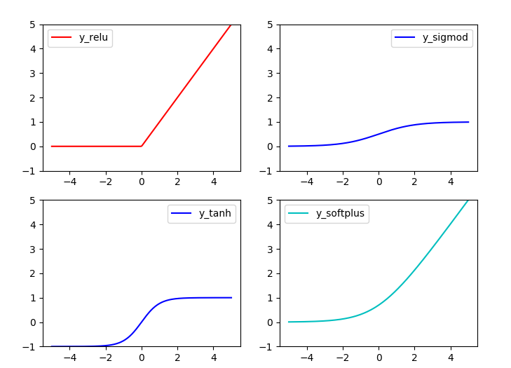
　　常用激励函数有(ref2): tanh, relu, sigmod, softplus

　　激励函数在TensorFlow代码实现：

#!/usr/bin/python

'''
Show the most used activation functions in Network
'''

import tensorflow as tf
import numpy as np
import matplotlib.pyplot as plt

x = np.linspace(-5, 5, 200)

#1. struct
#following are popular activation functions
y_relu = tf.nn.relu(x)
y_sigmod = tf.nn.sigmoid(x)
y_tanh = tf.nn.tanh(x)
y_softplus = tf.nn.softplus(x)

#2. session
sess = tf.Session()
y_relu, y_sigmod, y_tanh, y_softplus =sess.run([y_relu, y_sigmod, y_tanh, y_softplus])

# plot these activation functions
plt.figure(1, figsize=(8,6))

plt.subplot(221)
plt.plot(x, y_relu, c ='red', label = 'y_relu')
plt.ylim((-1, 5))
plt.legend(loc = 'best')

plt.subplot(222)
plt.plot(x, y_sigmod, c ='b', label = 'y_sigmod')
plt.ylim((-1, 5))
plt.legend(loc = 'best')

plt.subplot(223)
plt.plot(x, y_tanh, c ='b', label = 'y_tanh')
plt.ylim((-1, 5))
plt.legend(loc = 'best')

plt.subplot(224)
plt.plot(x, y_softplus, c ='c', label = 'y_softplus')
plt.ylim((-1, 5))
plt.legend(loc = 'best')

plt.show()

　结果：

　　　　　　　　

创建神经网络

　　创建层

　　定义函数用于创建隐藏层/输出层：　

#add a layer and return outputs of the layer
def add_layer(inputs, in_size, out_size, activation_function=None):
    #1. initial weights[in_size, out_size]
    Weights = tf.Variable(tf.random_normal([in_size,out_size]))
    #2. bias: (+0.1)
    biases = tf.Variable(tf.zeros([1,out_size]) + 0.1)
    #3. input*Weight + bias
    Wx_plus_b = tf.matmul(inputs, Weights) + biases
    #4. activation
    if activation_function is None:
        outputs = Wx_plus_b
    else:
        outputs = activation_function(Wx_plus_b)
    return outputs 

　　定义网络结构

　　此处定义一个三层网络，即：输入-单层隐藏层-输出层。可通过以上函数添加层数。网络为全连接网络。

# add hidden layer
l1 = add_layer(xs, 1, 10, activation_function=tf.nn.relu)
# add output layer
prediction = add_layer(l1, 10, 1, activation_function=None)

　　训练

　　利用梯度下降，训练1000次。

loss function: suqare error
loss = tf.reduce_mean(tf.reduce_sum(tf.square(ys - prediction), reduction_indices=[1]))
GD = tf.train.GradientDescentOptimizer(0.1)
train_step = GD.minimize(loss)

完整代码

#!/usr/bin/python

'''
Build a simple network
'''

import tensorflow as tf
import numpy as np

#1. add_layer
def add_layer(inputs, in_size, out_size, activation_function=None):
    #1. initial weights[in_size, out_size]
    Weights = tf.Variable(tf.random_normal([in_size,out_size]))
    #2. bias: (+0.1)
    biases = tf.Variable(tf.zeros([1,out_size]) + 0.1)
    #3. input*Weight + bias
    Wx_plus_b = tf.matmul(inputs, Weights) + biases
    #4. activation
    ## when activation_function is None then outlayer
    if activation_function is None:
        outputs = Wx_plus_b
    else:
        outputs = activation_function(Wx_plus_b)
    return outputs

##begin build network struct##
##network: 1 * 10 * 1
#2. create data
x_data = np.linspace(-1, 1, 300)[:, np.newaxis]
noise = np.random.normal(0, 0.05, x_data.shape)
y_data = np.square(x_data) - 0.5 + noise

#3. placehoder: waiting for the training data
xs = tf.placeholder(tf.float32, [None, 1])
ys = tf.placeholder(tf.float32, [None, 1])

#4. add hidden layer
h1 = add_layer(xs, 1, 10, activation_function=tf.nn.relu)
h2 = add_layer(h1, 10, 10, activation_function=tf.nn.relu)
#5. add output layer
prediction = add_layer(h2, 10, 1, activation_function=None)

#6. loss function: suqare error
loss = tf.reduce_mean(tf.reduce_sum(tf.square(ys - prediction), reduction_indices=[1]))
GD = tf.train.GradientDescentOptimizer(0.1)
train_step = GD.minimize(loss)
## End build network struct ###

## Initial the variables
if int((tf.__version__).split('.')[1]) < 12 and int((tf.__version__).split('.')[0]) < 1:
    init = tf.initialize_all_variables()
else:
    init = tf.global_variables_initializer()

## Session
sess = tf.Session()
sess.run(init)

# called in the visual

## Traing
for step in range(1000):
    #当运算要用到placeholder时，就需要feed_dict这个字典来指定输入
    sess.run(train_step, feed_dict={xs:x_data, ys:y_data})
    if i % 50 == 0:
        # to visualize the result and improvement
        try:
            ax.lines.remove(lines[0])
        except Exception:
            pass
        prediction_value = sess.run(prediction, feed_dict={xs: x_data})
        # plot the prediction
        lines = ax.plot(x_data, prediction_value, 'r-', lw=5)
        plt.pause(1)

sess.close()

结果：

　　　　　　

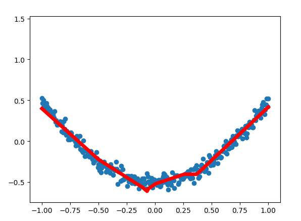
至此TensorFlow简易学习完结。

--------------------------------------

说明：本列为前期学习时记录，为基本概念和操作，不涉及深入部分。文字部分参考在文中注明，代码参考莫凡