Self-Taught Learning

the promise of self-taught learning and unsupervised feature learning is that if we can get our algorithms to learn from unlabeled data, then we can easily obtain and learn from massive amounts of it.Even though a single unlabeled example is less informative than a single labeled example, if we can get tons of the former---for example, by downloading random unlabeled images/audio clips/text documents off the internet---and if our algorithms can exploit this unlabeled data effectively, then we might be able to achieve better performance than the massive hand-engineering and massive hand-labeling approaches.

Learning features

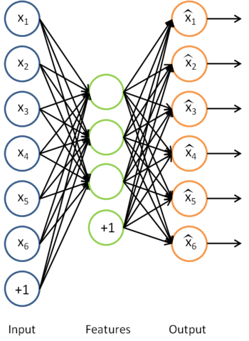
We have already seen how an autoencoder can be used to learn features from unlabeled data. Concretely, suppose we have an unlabeled training set with unlabeled examples. (The subscript "u" stands for "unlabeled.") We can then train a sparse autoencoder on this data (perhaps with appropriate whitening or other pre-processing):

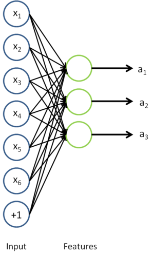
Having trained the parameters of this model, given any new input , we can now compute the corresponding vector of activations of the hidden units. As we saw previously, this often gives a better representation of the input than the original raw input . We can also visualize the algorithm for computing the features/activations as the following neural network:

This is just the sparse autoencoder that we previously had, with with the final layer removed.

Now, suppose we have a labeled training set of examples. (The subscript "l" stands for "labeled.") We can now find a better representation for the inputs. In particular, rather than representing the first training example as , we can feed as the input to our autoencoder, and obtain the corresponding vector of activations . To represent this example, we can either just replace the original feature vector with . Alternatively, we can concatenate the two feature vectors together, getting a representation .

Thus, our training set now becomes (if we use the replacement representation, and use to represent the -th training example), or (if we use the concatenated representation). In practice, the concatenated representation often works better; but for memory or computation representations, we will sometimes use the replacement representation as well.

Finally, we can train a supervised learning algorithm such as an SVM, logistic regression, etc. to obtain a function that makes predictions on the values. Given a test example , we would then follow the same procedure: For feed it to the autoencoder to get . Then, feed either or to the trained classifier to get a prediction.

On pre-processing the data

During the feature learning stage where we were learning from the unlabeled training set , we may have computed various pre-processing parameters. For example, one may have computed a mean value of the data and subtracted off this mean to perform mean normalization, or used PCA to compute a matrix to represent the data as (or used PCA whitening or ZCA whitening). If this is the case, then it is important to save away these preprocessing parameters, and to use the same parameters during the labeled training phase and the test phase, so as to make sure we are always transforming the data the same way to feed into the autoencoder. In particular, if we have computed a matrix using the unlabeled data and PCA, we should keep the same matrix and use it to preprocess the labeled examples and the test data. We should not re-estimate a different matrix (or data mean for mean normalization, etc.) using the labeled training set, since that might result in a dramatically different pre-processing transformation, which would make the input distribution to the autoencoder very different from what it was actually trained on.

On the terminology of unsupervised feature learning

There are two common unsupervised feature learning settings, depending on what type of unlabeled data you have. The more general and powerful setting is the self-taught learning setting, which does not assume that your unlabeled data x_u has to be drawn from the same distribution as your labeled data x_l. The more restrictive setting where the unlabeled data comes from exactly the same distribution as the labeled data is sometimes called the semi-supervised learning setting. This distinctions is best explained with an example, which we now give.

Suppose your goal is a computer vision task where you'd like to distinguish between images of cars and images of motorcycles; so, each labeled example in your training set is either an image of a car or an image of a motorcycle. Where can we get lots of unlabeled data? The easiest way would be to obtain some random collection of images, perhaps downloaded off the internet. We could then train the autoencoder on this large collection of images, and obtain useful features from them. Because here the unlabeled data is drawn from a different distribution than the labeled data (i.e., perhaps some of our unlabeled images may contain cars/motorcycles, but not every image downloaded is either a car or a motorcycle), we call this self-taught learning.

In contrast, if we happen to have lots of unlabeled images lying around that are all images of either a car or a motorcycle, but where the data is just missing its label (so you don't know which ones are cars, and which ones are motorcycles), then we could use this form of unlabeled data to learn the features. This setting---where each unlabeled example is drawn from the same distribution as your labeled examples---is sometimes called the semi-supervised setting. In practice, we often do not have this sort of unlabeled data (where would you get a database of images where every image is either a car or a motorcycle, but just missing its label?), and so in the context of learning features from unlabeled data, the self-taught learning setting is more broadly applicable.

自学习 VS 半监督学习

半监督学习假设，未标记数据和已标记数据拥有相同的数据分布