[Hinton] Neural Networks for Machine Learning - Hopfield Nets and Boltzmann Machine

高大上的模型和理论。

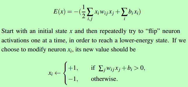
Hopfield Nets

看了能量函数，发现：

These look very much like the weights and biases of a neural network.

【点到为止】

Boltzmann machine learning

From: A Beginner’s Tutorial for Restricted Boltzmann Machines

Frankly, 这玩意晦涩难懂，且在卷积神经网络的大趋势下，工业界并没有什么优势，那又何必华这么大的力气在此呢？

Each visible node takes a low-level feature from an item in the dataset to be learned. For example, from a dataset of grayscale images, each visible node would receive one pixel-value for each pixel in one image. (MNIST images have 784 pixels, so neural nets processing them must have 784 input nodes on the visible layer.)

Now let’s follow that single pixel value, x, through the two-layer net. At node 1 of the hidden layer, x is multiplied by a weight and added to a so-called bias. The result of those two operations is fed into an activation function, which produces the node’s output, or the strength of the signal passing through it, given input x.

activation f((weight w * input x) + bias b ) = output a

Next, let’s look at how several inputs would combine at one hidden node. Each x is multiplied by a separate weight, the products are summed, added to a bias, and again the result is passed through an activation function to produce the node’s output.

Because inputs from all visible nodes are being passed to all hidden nodes, an RBM can be defined as a symmetrical bipartite graph. 【目前为止，与全连接相比没有太大新意】

Symmetrical means that each visible node is connected with each hidden node (see below). Bipartite means it has two parts, or layers, and the graph is a mathematical term for a web of nodes.

At each hidden node, each input x is multiplied by its respective weight w. That is, a single input x would have three weights here, making 12 weights altogether (4 input nodes x 3 hidden nodes). The weights between two layers will always form a matrix where the rows are equal to the input nodes, and the columns are equal to the output nodes.

Each hidden node receives the four inputs multiplied by their respective weights. The sum of those products is again added to a bias (which forces at least some activations to happen), and the result is passed through the activation algorithm producing one output for each hidden node.

If these two layers were part of a deeper neural network, the outputs of hidden layer no. 1 would be passed as inputs to hidden layer no. 2, and from there through as many hidden layers as you like until they reach a final classifying layer. (For simple feed-forward movements, the RBM nodes function as an autoencoder and nothing more.)

【到此为止，暂无新事】

Reconstructions

But in this introduction to restricted Boltzmann machines, we’ll focus on how they learn to reconstruct data by themselves in an unsupervised fashion (unsupervised means without ground-truth labels in a test set), making several forward and backward passes between the visible layer and hidden layer no. 1 without involving a deeper network.

In the reconstruction phase, the activations of hidden layer no. 1 become the input in a backward pass. They are multiplied by the same weights, one per internode edge, just as x was weight-adjusted on the forward pass. The sum of those products is added to a visible-layer bias at each visible node, and the output of those operations is a reconstruction; i.e. an approximation of the original input. This can be represented by the following diagram:

Because the weights of the RBM are randomly initialized, the difference between the reconstructions and the original input is often large. You can think of reconstruction error as the difference between the values of r and the input values, and that error is then backpropagated against the RBM’s weights, again and again, in an iterative learning process until an error minimum is reached.

A more thorough explanation of backpropagation is here.

As you can see, on its forward pass, an RBM uses inputs to make predictions about node activations, or the probability of output given a weighted x: p(a|x; w).

But on its backward pass, when activations are fed in and reconstructions, or guesses about the original data, are spit out, an RBM is attempting to estimate the probability of inputs x given activations a, which are weighted with the same coefficients as those used on the forward pass. This second phase can be expressed as p(x|a; w).

Together, those two estimates will lead you to the joint probability distribution of inputs x and activations a, or p(x, a).

Reconstruction does something different from regression, which estimates a continous value based on many inputs, and different from classification, which makes guesses about which discrete label to apply to a given input example.

Reconstruction is making guesses about the probability distribution of the original input; i.e. the values of many varied points at once. This is known as generative learning, which must be distinguished from the so-called discriminative learning performed by classification, which maps inputs to labels, effectively drawing lines between groups of data points.

Let’s imagine that both the input data and the reconstructions are normal curves of different shapes, which only partially overlap.

To measure the distance between its estimated probability distribution and the ground-truth distribution of the input, RBMs use Kullback Leibler Divergence. A thorough explanation of the math can be found on Wikipedia.

KL-Divergence measures the non-overlapping, or diverging, areas under the two curves, and an RBM’s optimization algorithm attempts to minimize those areas so that the shared weights, when multiplied by activations of hidden layer one, produce a close approximation of the original input. On the left is the probability distibution of a set of original input, p, juxtaposed with the reconstructed distribution q; on the right, the integration of their differences.

【如何理解Boltzmann machine是生成式模型】

3. 深度信念网络（DBN）

深度信念网络（Deep Belief Network，DBN）是早期深度生成式模型的典型代表，它由多层神经元构成，这些神经元又分为可见神经元和隐性神经元，可见单元用于接受输入，隐单元用于提取特征。网络最顶上的两层间的连接是无向的，组成联合内存 (associative memory)，较低的其他层之间有连接上下的有向连接。最底层代表了数据向量 (data vectors)，每一个神经元代表数据向量的一维。

DBN的组成元件是受限玻尔兹曼机（Restricted Boltzmann Machines ,RBM）。单个RBM由两层网络组成：

一层叫做可见层 (visible layer)，由可见单元 (visible units) 组成，用于输入训练数据；
另一层叫做隐层 (Hidden layer)，由隐单元 (hidden units) 组成，用作特征检测器 (feature detectors)。

RBM既是一个生成模型，也是一个无监督模型，因为它使用隐变量来描述输入数据的分布，而且这个过程没有涉及数据的标签信息。单层RBM网络的学习目标是无监督地训练网络，使得可见层节点v的分布p(v)最大可能地拟合输入样本所在样本空间的真实分布q(v)。通过计算可见向量p(v)的对数似然log p(v)的梯度来更新RBM的权值【看样子既是局部输入也是局部输出】，这个计算过程涉及到了求解RBM模型所确定分布上的期望。

对于生成式模型概率推断过程中遇到的计算某分布下函数的期望、计算边缘概率分布等复杂问题，可以采用蒙特卡洛思想近似求解。

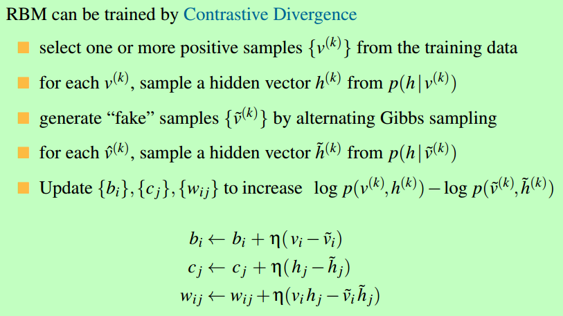
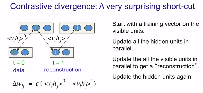
DBN采用对比散度（Contrastive Divergence, CD-k）算法，利用Gibbs采样的方法来估计RBM的对数似然梯度。

多个RBM堆叠组成一个DBN，将隐单元的激活概率（activation probabilities）作为下一层RBM的可见层输入数据，从底向上逐层预训练。DBN是一种生成模型，通过训练其神经元间的权重，我们可以让整个神经网络按照最大概率来生成训练数据。

生成样本时，使用训练好的随机隐单元状态值，首先在网络最顶两层进行多次Gibbs采样，生成该分布下的采样，然后向下传播，得到每层的状态和最终的样本。

训练

貌似有更好的改进，如下：