Image Super-Resolution via Sparse Representation——基于稀疏表示的超分辨率重建

　　经典超分辨率重建论文，基于稀疏表示。下面首先介绍稀疏表示，然后介绍论文的基本思想和算法优化过程，最后使用python进行实验。

稀疏表示

　　稀疏表示是指，使用过完备字典中少量向量的线性组合来表示某个元素。过完备字典是一个列数大于行数的行满秩矩阵，也就是说，它的列向量有无数种线性组合来表达列向量空间中的任意点。由于它的列数通常远大于行数，可以使用占比很小的列向量来表示特定的向量，我们称这种表示为稀疏表示。

　　那么如何获得这个字典呢？它在特定的任务下有特定的取值。和炼丹类似，我们先要用大量数据来训练这个矩阵，让它提取出能稀疏表示这些数据的特征，进而拥有稀疏表示其它相似数据的能力。

　　训练过完备字典的过程称为稀疏编码。设训练数据集为矩阵$X=(x_1,x_2,...,x_n)\in R^{m\times n}$，待训练矩阵为$A\in R^{m\times K}$，矩阵对每一数据的表示权重为$\alpha = (\alpha_1,\alpha_2,...,\alpha_n)\in R^{K\times n}$。进行如下优化：

\begin{align} \min\limits_{A,\alpha}\|\alpha\|_0\;\;\;s.t. \;  \|A\alpha - X\|_2^2\le \epsilon \end{align}

　　容易理解，约束重建向量与原始向量差异的同时，优化表示权重$\alpha$的稀疏性。通过优化获得所需的过完备字典后，我们就可以用它来稀疏表示新的数据了。对于某个向量$y$，我们可以进行类似的优化来获得它在字典中的稀疏表示：

\begin{align} \min\limits_{\alpha}\|\alpha\|_0\;\;\;s.t. \;  \|A\alpha - y\|_2^2\le \epsilon \end{align}

　　因为零范数的离散性，以上优化是NP-难问题，无法用正常的优化算法解决。所以通常会对上式进行调整，以方便优化。而在线性约束下，对一范数的优化有稀疏性（点击链接理解），因此可以转换为对一范数的优化。然后根据拉格朗日乘子法（据说如此，但我觉得这个转换并不等价），不等式约束可以移入优化中：

\begin{align} \min\limits_{\alpha} \lambda \|\alpha\|_1 + \|A\alpha - y\|_2^2 \end{align}

　　同样，$(1)$式也可以进行类似的转换。

　　以上就是稀疏表示的流程，看到这个提取特征然后重建的过程，我们会联想到主成分分析（PCA）。PCA能使我们方便地找到一组“完备”基向量，但是这里我们要做的是找到一组“过完备”的基向量来表示输入向量。过完备基的好处是它们能更有效地找出隐含在输入数据内部的结构与模式。然而，与PCA不同，对于过完备基来说，系数$\alpha$不再由输入向量$y$单独确定。因此，在稀疏编码算法中，我们另加一个评判标准“稀疏性”来解决因过完备而导致的退化（degeneracy）问题。

　　上面这段是百度百科原话。我觉得，把过完备字典与神经网络进行对比，可以把这个待训练的很“宽”的矩阵看做参数量很大的网络。我们知道参数量大而训练数据不充足的时候模型很容易过拟合，为了防止过拟合就要加上正则项，以使参数能专注于学习更有共性的特征。我们可以把上面的稀疏性看做正则化来理解，使字典的列向量能表达一些更有“特点”的信息。

论文原理及实现流程

基本思想

　　在训练阶段，论文同时对LR训练集$Y= (y_1,y_2,...,y_n)$和对应的HR训练集$X = (x_1,x_2,...,x_n)$分别训练两个过完备字典$D_l,D_h$，使得LR数据$y_i$和它对应的HR数据$x_i$能以相同的稀疏编码$\alpha_i$分别被$D_l$和$D_h$表示。也就是

$\left\{ \begin{aligned} &D_l\alpha_i \approx y_i \\ &D_h\alpha_i \approx x_i \end{aligned} \right.$

　　在测试阶段，我们已经有了训练好的$D_l$和相对应的$D_h$。对于测试图像$y_t$，首先通过优化获得$y_t$在$D_l$中的稀疏表示$\alpha_t$，此时有$D_l\alpha_t \approx y_t$。然后用这个表示通过$D_h$映射出对应的SR图像，即$\hat{x}_t=D_h\alpha_t$。

训练过程

　　训练过程就是训练上述的过完备字典对。因为性能的因素，我们不可能直接对整张图进行稀疏编码，论文是将图像分为方形的区块（patch）进行编码的。因此，用于训练的成对数据不是整张的LR-HR图像对，而是所有图像分割开来的区块对。现在把LR训练集的所有区块表示为$Y=(y_1,y_2,...,y_n)\in R^{M\times n}$，相应的HR训练集区块表示为$X = (x_1,x_2,...,x_n)\in R^{N\times n}$。如果放大倍数为$t$倍，则有$N=t^2M$。

　　优化式很直观：

\begin{align} \min\limits_{D_l,D_h,\alpha}\frac{1}{N}\|X - D_h\alpha\|_2^2+\frac{1}{M}\|Y - D_l\alpha\|_2^2 + \lambda \|\alpha\|_1 \end{align}

　　其中$D_l\in R^{M\times K},D_h\in R^{N\times K}$，分别表示待训练的LR和HR字典，$K$表示字典的原子数；$\alpha\in R^{K\times n}$为表示矩阵；$\lambda$为平衡稀疏性和重建一致性的系数。一二两项惩罚使用相同表示的重建差异，第三项用来优化表示的稀疏性。把前两项合并，可得：

\begin{aligned} \min\limits_{D_c,\alpha}\|X_c - D_c\alpha\|_2^2 + \lambda \|\alpha\|_1 \end{aligned}

　　其中

$X_c = \left[ \begin{aligned} &\frac{1}{\sqrt{N}}X\\ &\frac{1}{\sqrt{M}}Y \end{aligned} \right], D_c = \left[ \begin{aligned} &\frac{1}{\sqrt{N}}D_h\\ &\frac{1}{\sqrt{M}}D_l \end{aligned} \right]$

　　论文说同时优化$D_c$和$\alpha$非凸，但是固定其中一个变量，然后对另一个变量的优化则是凸的。因此可以将凸优化交替进行，最终可以达到一个局部最优点。然而我还是选择无脑梯度下降算了。当然我们可以使用SGD，每次随机选择部分区块执行迭代，这样做的好处在于可以引入随机性从而增加跳出局部最优的可能性。引人注意的是，执行SGD时，待优化的权重是$D_c$和$\alpha$，但由于每次只选择部分区块，$\alpha$也只能选择对应的那部分进行更新，这有点像Dropout。但是，后面实验的时候发现，SGD的效果并没有GD好，因此没有分成小批量来迭代。

推理过程

　　在获得$D_l$和$D_h$后，就可以用它们对LR图像进行重建了。论文采用扫描的方式，一个区块一个区块从上到下、从左到右对测试图像进行超分辨率重建。另外，为了使相邻区块之间能相互匹配，防止颜色上的冲突，前后两个区块之间设有重叠部分，在重建一个区块时，重叠部分要和上一个区块一致。具体优化方式如下。

　　首先将测试图像$y$按顺序划分为$m$个区块$(p_1,p_2,...,p_m)$，设区块在$D_l$中的表示为$(\alpha_1,\alpha_2,...,\alpha_m)$。按顺序对所有区块执行优化，对于第$i$个区块，优化式如下：

\begin{align} \min\limits_{\alpha_i} \lambda\|\alpha_i\|_1 + \|FD_l\alpha_i - Fp_i\|_2^2+ \|PD_h\alpha_i - w\|_2^2 \end{align}

　　其中$w$表示已重建区块和当前区块的重叠部分，$P$表示将当前区块映射为重叠部分的矩阵。至于$F$，论文说是一个线性提取器，使图像中感知效果更好。论文实验时用的是一阶、二阶导数滤波器，但没说清楚具体如何操作，我实验就没有用。

　　式子意义很明显，第一项保证表示的稀疏性，第二项优化原始LR图像的重建一致性，第三项优化SR图像相邻区块重叠部分的一致性。获得SR图像所有区块的稀疏表示后，左乘$D_h$，然后将区块拼接起来，就是最终的SR图像了。

　　除了以上步骤以外，论文还多了一个所谓全局重建约束。用什么反向投影法，通过迭代让SR图像退化后能和原始图像更相似。由于说的很不清楚，这里就不加了，而且我觉得这不是这篇论文的主要内容。

　　另外，论文在执行推理过程之前，先将原图减去自身元素的均值，以使模型能更专注于纹理的重建，在重建完的SR图像上再加回这个均值。但是这个策略只在推理章节提了一句，在训练$D_l,D_h$时是否使用标准化的图像并没有说明。

实验与分析

　　实验使用LSUN数据集中的bedroom作为训练集，从中选取1024张长宽都大于256像素的图片，居中裁剪至256x256，获得HR训练集。然后对HR使用Bicubic缩小4倍至64x64，获得LR训练集。将LR区块划分为4x4大小，HR区块划分为16x16大小，则每张图片都可被划分为16x16个区块。另外定义$D_l$和$D_h$的原子（列向量）数为2560（算力有限），又由于彩色图片有三个通道，因此$D_l$和$D_h$的列向量长度分别为$4\times 4 \times 3$和$16\times 16 \times 3$。

训练

　　综上，对于$(4)$式中的各个参数，有：

\begin{equation} \left\{ \begin{aligned} &X \in R^{(16\times 16\times 3)\times (1024\times 16^2)}\\ &Y \in R^{(4\times 4\times 3)\times (1024\times 16^2)}\\ &D_h \in R^{(16\times 16\times 3)\times 2560}\\ &D_l \in R^{(4\times 4\times 3)\times 2560}\\ &\alpha \in R^{2560\times (1024\times 16^2)}\\ \end{aligned} \right. \end{equation}

　　另设$(4)$式$\lambda=0.1$，使用RMSProp对$(4)$式进行优化，根据以上所列参数，Pytorch代码如下：

#%%
import torch,os
import numpy as np
import matplotlib.pyplot as plt
from torch import optim,cuda

#读取图像
LR_path = r'E:\DataSets\SRTest\LR'
HR_path = r'E:\DataSets\SRTest\HR'
LR_imgs = np.zeros([1024,64,64,3])
HR_imgs = np.zeros([1024,256,256,3])

for i, j in zip(os.listdir(LR_path),range(1024)):
  img_path = os.path.join(LR_path,i)
  LR_imgs[j] = plt.imread(img_path)/255
for i, j in zip(os.listdir(HR_path),range(1024)):
  img_path = os.path.join(HR_path,i)
  HR_imgs[j] = plt.imread(img_path)/255

#定义各个变量
def imgs2patches(imgs, patch_size):
  #将图像集转换为区块集
  imgs_n = len(imgs)
  patch_n = int(imgs.shape[1]/patch_size)
  patches = np.zeros([imgs_n*patch_n**2, patch_size*patch_size*3])
  for i in range(patch_n):
    for j in range(patch_n):
      t = imgs[:,i*patch_size:(i+1)*patch_size,j*patch_size:(j+1)*patch_size,:]
      t = np.reshape(t,[imgs_n,-1])
      now = i * patch_n + j
      patches[imgs_n*now:imgs_n*(now+1),:] = t
  return patches.T

atom_n = 2560

X = torch.tensor(imgs2patches(HR_imgs, 16),device='cuda')*255 #训练集图像元素色值取值在[0,255]
Y = torch.tensor(imgs2patches(LR_imgs, 4), device='cuda')*255
Dh = torch.normal(0,1,[16*16*3,atom_n],device='cuda')
Dl = torch.normal(0,1,[4*4*3,atom_n],device='cuda') 

alpha = torch.normal(0,1,[atom_n,1024*16*16],device='cuda')
Dh.requires_grad_(True)
Dl.requires_grad_(True)
alpha.requires_grad_(True)
opt = optim.RMSprop([Dh,Dl,alpha])
#%%
#训练模型
from torch.utils.tensorboard import SummaryWriter 

writer = SummaryWriter('logs/')
def iter_one_epoch(lamb=0.01):
  patch_n = alpha.shape[1]
  term1 = torch.sum((X - torch.matmul(Dh,alpha))**2)/256/patch_n
  term2 = torch.sum((Y - torch.matmul(Dl,alpha))**2)/16/patch_n
  term3 = lamb * torch.sum(torch.abs(alpha))/patch_n
  loss = term1 + term2 + term3
  opt.zero_grad()
  loss.backward()
  opt.step()
  return term1,term2,term3,loss

for i in range(1, 1500):
  term1,term2,term3,loss = iter_one_epoch(lamb=0.1)
  print(i,loss.cpu().detach().numpy())
  writer.add_scalar('term1', term1, int(i))
  writer.add_scalar('term2', term2, int(i))
  writer.add_scalar('term3', term3, int(i))
  writer.add_scalar('loss', loss, int(i))
  if i % 700 == 0:
    for i in opt.param_groups:
      i['lr'] = i['lr']*0.5
print("保存字典")
torch.save(Dl,'dictionaries/Dic_LR')#保存两个字典
torch.save(Dh,'dictionaries/Dic_HR')
#%%
#用Dh重建HR图像验证训练结果
def get_recon_LR_HR(n):
  print(Dh.shape,Dl.shape)

  recon_LR = torch.matmul(Dl, alpha)
  recon_HR = torch.matmul(Dh, alpha)
  LR = torch.zeros([1024,64,64,3],device='cuda')
  HR = torch.zeros([1024,256,256,3],device='cuda') 

  for i in range(n):
    print(i)
    for j in range(16):
      for k in range(16):
        LR[i,4*j:4*(j+1),4*k:4*(k+1),:] = recon_LR[:,i+(j*16+k)*1024].reshape([4,4,3])
        HR[i,16*j:16*(j+1),16*k:16*(k+1),:] = recon_HR[:,i+(j*16+k)*1024].reshape([16,16,3])
  return LR,HR
lr,hr = get_recon_LR_HR(100)
n = 10
fig = plt.figure(figsize=(15,15))
ax1,ax2,ax3,ax4 = fig.add_subplot(221),fig.add_subplot(222),fig.add_subplot(223),fig.add_subplot(224)
ax1.imshow(LR_imgs[n])
ax2.imshow(lr[n].cpu().detach()/255)
ax3.imshow(HR_imgs[n])
ax4.imshow(hr[n].cpu().detach()/255)
ax1.set_title('LR image',fontsize=20)
ax2.set_title('Reconstructed LR image',fontsize=20)
ax3.set_title('HR image',fontsize=20)
ax4.set_title('Reconstructed HR image',fontsize=20)
plt.show()   

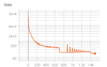
　　我另外对比过Adam和原始GD，迭代速度都没有RMSProp快，而且loss在稳定后是最小的。算法总共迭代了1500次，使用的是RMSProp默认的学习率，但每700次迭代都会下调为原来的一半。整个迭代在3090下用时10分钟，loss变化如下：

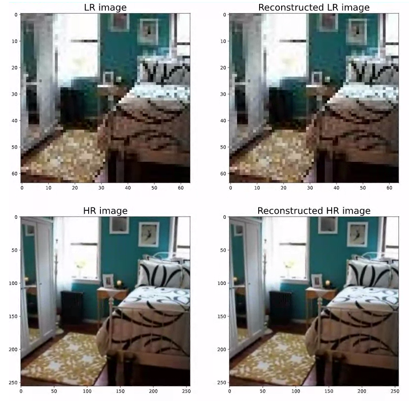
　　以下是训练集的LR和它对应的HR图像的重建效果，几乎看不出差异：

推理

顺序优化区块

　　论文的推理策略是按顺序重建SR图像的各个区块，同时约束相邻区块的重叠部分的相似性。定义LR图像相邻区块之间的重叠为1像素宽，则相应SR图像相邻区块之间有4像素宽的重叠，并且图像能分成21x21个区块。则$(5)$式各个变量的规模如下

\begin{equation} \left\{ \begin{aligned} &\alpha_{ij}\in R^{2560\times 1},\;\;i,j=1,2,...,21\\ &p_{ij}\in R^{(4\times 4\times 3) \times 1},\;\;i,j=1,2,...,21\\ &D_l\in R^{(4\times 4\times 3) \times2560}\\ &D_h\in R^{(16\times 16\times 3) \times 2560}\\ \end{aligned} \right. \end{equation}

　　优化代码如下：

#%%
import torch
import matplotlib.pyplot as plt
from torch import optim
from torch import random
from torch.nn import functional as F

path_lr = r'E:\DataSets\SRTest\TestImages\LR\0003.jpg'
path_hr = r'E:\DataSets\SRTest\TestImages\HR\0003.jpg'
img_lr = plt.imread(path_lr)
img_hr = plt.imread(path_hr) 

Dl = torch.load('dictionaries/Dic_LR').reshape([4,4,3,2560])
Dh = torch.load('dictionaries/Dic_HR').reshape([16,16,3,2560])
def img_SR(LR_img, lambda1=0.5,lambda2=1,lambda3=1,lambda4=1,epoch=100):
  '''
  LR_img取值须在[0,255],形状为[64,64,3]
  '''
  LR_img = torch.tensor(LR_img,device='cuda',requires_grad=False)
  SR_img = torch.zeros([256,256,3],device='cuda',requires_grad=False) 

  alpha_array = []
  for i in range(21):
    al = []
    for j in range(21):
      al.append(torch.normal(0,1,[2560],device='cuda',requires_grad=True))
    alpha_array.append(al)

  def SRcompat_loss(patch, i, j):
    loss = 0
    if i > 0:
      loss += torch.mean(torch.abs(SR_img[12*i:12*i+4,12*j:12*j+16] - patch[:4]))
    if j > 0:
      loss += torch.mean(torch.abs(SR_img[12*i:12*i+16,12*j:12*j+4] - patch[:,:4]))
    return loss

  #按顺序计算SR各个区块
  for i in range(21):
    for j in range(21):
      alpha = alpha_array[i][j]
      opt = optim.RMSprop([alpha])
      for k in range(1, epoch):
        L1 = torch.mean(torch.abs(alpha))
        L2 = torch.mean(torch.abs(torch.matmul(Dl,alpha) - LR_img[i*3:i*3+4,j*3:j*3+4]))
        L3 = SRcompat_loss(torch.matmul(Dh,alpha), i, j)
        down_SR = F.interpolate(torch.matmul(Dh,alpha).reshape([1,16,16,3]).permute([0,3,1,2]),size=[4,4], mode='bicubic')
        L4 = torch.mean(torch.abs(down_SR[0].permute([1,2,0]) - LR_img[i*3:i*3+4,j*3:j*3+4]))#额外的下采样一致性
        Loss = lambda1 * L1 + lambda2 * L2 + lambda3 * L3 + lambda4 * L4
        if k%800 ==0:
          print(k,Loss)
          for l in opt.param_groups:
            l['lr'] *= 0.5
        opt.zero_grad()
        Loss.backward()
        opt.step()
        if Loss < 5:
          print(k,Loss)
          break
      SR_img[12*i:12*i+16,12*j:12*j+16] = torch.matmul(Dh,alpha).detach()
    plt.imshow(SR_img.detach().cpu()/255)
    plt.show()
  return SR_img

img_sr = img_SR(img_lr,0.01,1,1,1,5000).cpu()/255
fig = plt.figure(figsize=(15,15))
ax1,ax2,ax3 = fig.add_subplot(131),fig.add_subplot(132),fig.add_subplot(133)
ax1.imshow(img_lr),ax1.set_title('LR',fontsize=20)
ax2.imshow(img_sr),ax2.set_title('SR',fontsize=20)
ax3.imshow(img_hr),ax3.set_title('HR',fontsize=20)
plt.show()

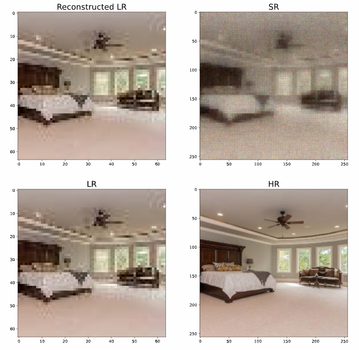
　　迭代了好久，结果如下：

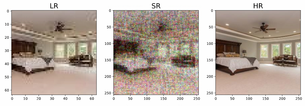
　　噪声很多，原因应该就是没有用论文中提到的使用反向投影法进行精炼，以及使用$F$操作吧。

另一种推理方式

　　由于上述优化有先后顺序，后面的区块可能会损失精读来“迁就”前面已获得的SR区块，让重叠部分一致。因此论文在完成这一步后又加了一个全局一致性的约束，来调整已获得的SR图像，就是用所谓的反向投影法，但是写得很不明白。因此，我试验了一种直接对所有区块同时进行优化的方法。

　　首先定义LR图像相邻区块的重叠为2像素宽，也就是4x4区块的一半。则相应的SR图像的相邻区块重叠为8像素宽，同样占其区块的一半。如此一来，SR相邻区块的兼容性可以通过创建两个“补丁”图来约束，如下图所示：

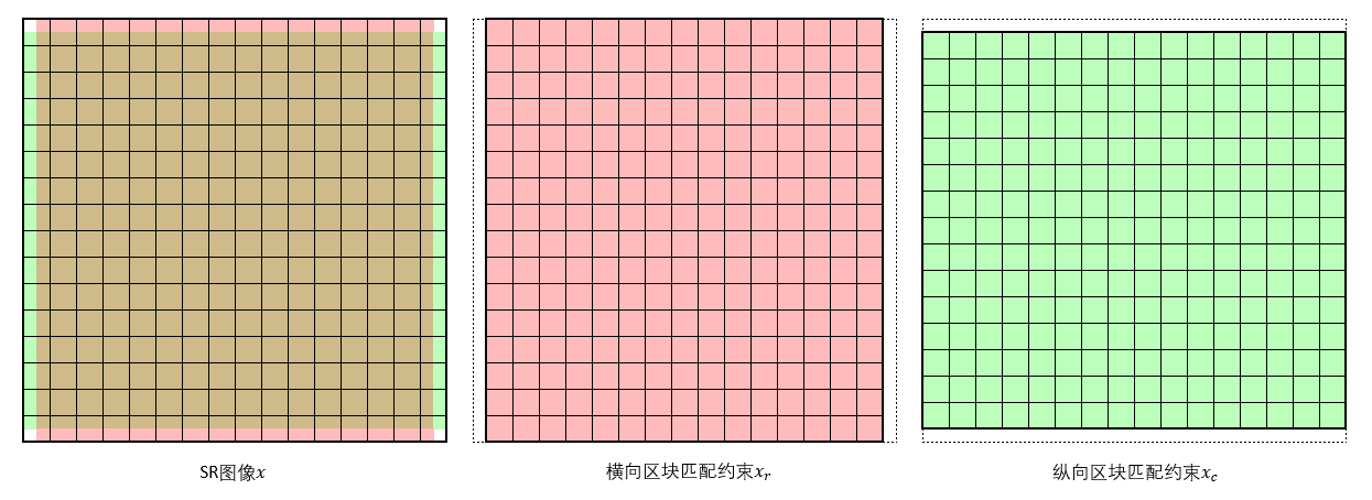
　　即同时优化三个SR图像，第一张是最终的SR结果$x$，第二张用于约束$x$横向相邻区块之间的匹配度，第三张用于约束$x$纵向相邻区块之间的匹配度。也就是说，第一张图像相邻区块各取一半拼接成的图块要与第二、三图像中对应的区块一致。

　　综上，对于测试LR图像$y$，分别去掉左右、上下边缘的2像素宽、高的图块，获得用于匹配约束的$y_r,y_c$。然后分别定义相应的表示$\alpha,\alpha_r,\alpha_c$。根据以上定义，各个参数的规模如下（LR图像区块被展开为向量的形式）：

\begin{equation} \left\{ \begin{aligned} &\alpha\in R^{2560\times (16\times 16)}\\ &\alpha_r\in R^{2560\times (16\times 15)}\\ &\alpha_c\in R^{2560\times (15\times 16)}\\ &y\in R^{(4\times 4\times 3) \times(16\times 16)}\\ &y_r\in R^{(4\times 4\times 3) \times(16\times 15)}\\ &y_c\in R^{(4\times 4\times 3) \times(15\times 16)}\\ &D_l\in R^{(4\times 4\times 3) \times2560}\\ &D_h\in R^{(16\times 16\times 3) \times 2560}\\ \end{aligned} \right. \end{equation}

　　则稀疏性约束、重建一致性约束、区块匹配度约束和最终的优化式如下：

\begin{equation} \begin{aligned} &L_{spars} = \|\alpha\|_1+\|\alpha_r\|_1+\|\alpha_c\|_1  \\ &L_{recon} = \|D_l\alpha - y\|_1+\|D_l\alpha_r - y_r\|_1+\|D_l\alpha_c - y_c\|_1 \\ &L_{comp} = \|P_1D_h\alpha - D_h\alpha_r\|_1+\|P_2D_h\alpha - D_h\alpha_c\|_1\\ &\min\limits_{\alpha,\alpha_r,\alpha_c}Loss =  \lambda_1 L_{spars}+\lambda_2L_{recon}+\lambda_3L_{comp} \end{aligned} \end{equation}

　　$P_1,P_2$表示将SR图像映射到相应的匹配约束图像的操作，$\lambda_1,\lambda_2,\lambda_3$用于平衡三个约束的占比。使用$L1$范数是因为它能生成噪声更少的图像。另外，为了防止梯度过大，代码中计算的各项范数会除以元素数量，公式中没有标明。代码如下：

#%%
import torch
import matplotlib.pyplot as plt
from torch import optim
from torch.utils.tensorboard import SummaryWriter 

path_lr = r'E:\DataSets\SRTest\TestImages\LR\0003.jpg'
path_hr = r'E:\DataSets\SRTest\TestImages\HR\0003.jpg'
img_lr = plt.imread(path_lr)
img_hr = plt.imread(path_hr) 

Dl = torch.load('dictionaries/Dic_LR')
Dh = torch.load('dictionaries/Dic_HR')
def img_SR(LR_img, lambda1=0.5,lambda2=1,lambda3=1,epoch=100):
  '''
  LR_img取值须在[0,255],形状为[64,64,3]
  '''
  LR_img = torch.tensor(LR_img,device='cuda',dtype=torch.float32)
  LR_img_r = LR_img[:,2:-2]
  LR_img_c = LR_img[2:-2,:]
  def img2patches(img):
    patch_r = int(img.shape[0]/4)
    patch_c = int(img.shape[1]/4)
    patches = torch.zeros([4*4*3, patch_r*patch_c],device='cuda')
    for i in range(patch_r):
      for j in range(patch_c):
        patches[:,i * patch_c + j] = torch.flatten(img[i*4:(i+1)*4,j*4:(j+1)*4])
    return patches
  def patches2img(patches,row,col,ps=16):
    img = torch.zeros([row*ps, col*ps, 3],device='cuda')
    for i in range(row):
      for j in range(col):
        img[i*ps:(i+1)*ps, j*ps:(j+1)*ps] = patches[:,i*col+j].reshape([ps,ps,3])
    return img

  alpha = torch.normal(0,1,[2560,16*16],requires_grad=True,device='cuda')
  alpha_r = torch.normal(0,1,[2560,16*15],requires_grad=True,device='cuda')
  alpha_c = torch.normal(0,1,[2560,15*16],requires_grad=True,device='cuda')
  y = img2patches(LR_img)
  y_r = img2patches(LR_img_r)
  y_c = img2patches(LR_img_c) 

  opt = optim.RMSprop([alpha,alpha_r,alpha_c])

  writer = SummaryWriter('InferLogs2/')
  for i in range(1, epoch):
    l_alpha = torch.mean(torch.abs(alpha))
    l_alpha_r = torch.mean(torch.abs(alpha_r))
    l_alpha_c = torch.mean(torch.abs(alpha_c))
    L1 = l_alpha + l_alpha_r + l_alpha_c

    l_rec1 = torch.mean(torch.abs(torch.matmul(Dl,alpha)-y))
    l_rec2 = torch.mean(torch.abs(torch.matmul(Dl,alpha_r)-y_r))
    l_rec3 = torch.mean(torch.abs(torch.matmul(Dl,alpha_c)-y_c))
    L2 = l_rec1 + l_rec2 + l_rec3

    l_comp1 = torch.mean(torch.abs(patches2img(torch.matmul(Dh,alpha),16,16,16)[:,8:-8] - patches2img(torch.matmul(Dh,alpha_r),16,15,16)))
    l_comp2 = torch.mean(torch.abs(patches2img(torch.matmul(Dh,alpha),16,16,16)[8:-8,:] - patches2img(torch.matmul(Dh,alpha_c),15,16,16)))
    L3 = l_comp1 + l_comp2

    Loss = lambda1 * L1 + lambda2 * L2 + lambda3 * L3

    opt.zero_grad()
    Loss.backward()
    opt.step()

    writer.add_scalar('L1',L1,i)
    writer.add_scalar('L2',L2,i)
    writer.add_scalar('L3',L3,i)
    writer.add_scalar('Loss',Loss,i)
    if i % 50 == 0:
      print(i, Loss)
      plt.imshow(patches2img(torch.matmul(Dh,alpha),16,16,16).detach().cpu()/255)
      plt.show()
      plt.imshow(patches2img(torch.matmul(Dl,alpha),16,16,4).detach().cpu()/255)
      plt.show()
    if i % 300 == 0:
      for i in opt.param_groups:
        i['lr'] *= 0.5 

  return patches2img(torch.matmul(Dl,alpha),16,16,4),patches2img(torch.matmul(Dh,alpha),16,16,16)
recon_LR_img,SR_img = img_SR(img_lr,100,1,1,epoch=1500)
fig = plt.figure(figsize=(15,15))
ax1,ax2,ax3,ax4 = fig.add_subplot(221),fig.add_subplot(222),fig.add_subplot(223),fig.add_subplot(224)
ax1.imshow(recon_LR_img.detach().cpu()/255),ax1.set_title('Reconstructed LR',fontsize=20)
ax2.imshow(SR_img.detach().cpu()/255),ax2.set_title('SR',fontsize=20)
ax3.imshow(img_lr),ax3.set_title('LR',fontsize=20)
ax4.imshow(img_hr),ax4.set_title('HR',fontsize=20)
plt.show()

　　不过实际效果也并不是很好：

总结

　　综上，单纯使用稀疏表示做SR效果并不如人意。因为论文中还加了其它的方式和技巧来减少重建图像的噪声，而我这个实验没有加入，并且，论文的实验是放大3倍，区块大小为3x3，我这里与其并不相同，所以没能重现出论文的效果。另外，还可能是优化算法的缘故，论文使用的是凸优化（可能有某种方式算出解析解，但我看到L1范数就放弃了），我则是梯度下降。

　　主要还是不想再做了。。。论文作者没有给出源代码，自己敲代码加写博客用了4天时间，想看其它论文了。

论文地址

　　Image Super-Resolution via Sparse Representation