LOGIT REGRESSION

Version info: Code for this page was tested in SPSS 20.

Logistic regression, also called a logit model, is used to model dichotomous outcome variables. In the logit model the log odds of the outcome is modeled as a linear combination of the predictor variables.

Please note: The purpose of this page is to show how to use various data analysis commands. It does not cover all aspects of the research process which researchers are expected to do. In particular, it does not cover data cleaning and checking, verification of assumptions, model diagnostics and potential follow-up analyses.

Examples

Example 1: Suppose that we are interested in the factors

that influence whether a political candidate wins an election. The

outcome (response) variable is binary (0/1); win or lose.

The predictor variables of interest are the amount of money spent on the campaign, the

amount of time spent campaigning negatively and whether or not the candidate is an

incumbent.

Example 2: A researcher is interested in how variables, such as GRE (Graduate Record Exam scores),

GPA (grade

point average) and prestige of the undergraduate institution, effect admission into graduate

school. The response variable, admit/don’t admit, is a binary variable.

Description of the data

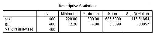
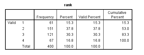
For our data analysis below, we are going to expand on Example 2 about getting into graduate school. We have generated hypothetical data, which can be obtained from our website by clicking on binary.sav. You can store this anywhere you like, but the syntax below assumes it has been stored in the directory c:data. This dataset has a binary response (outcome, dependent) variable called admit, which is equal to 1 if the individual was admitted to graduate school, and 0 otherwise. There are three predictor variables: gre, gpa, and rank. We will treat the variables gre and gpa as continuous. The variable rank takes on the values 1 through 4. Institutions with a rank of 1 have the highest prestige, while those with a rank of 4 have the lowest. We start out by opening the dataset and looking at some descriptive statistics.

get file = "c:databinary.sav".

descriptives /variables=gre gpa.


frequencies /variables = rank.


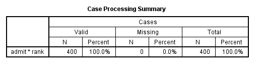
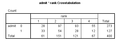
crosstabs /tables = admit by rank.

Analysis methods you might consider

Below is a list of some analysis methods you may have encountered. Some of the methods listed are quite reasonable while others have either fallen out of favor or have limitations.

Logistic regression, the focus of this page.
Probit regression. Probit analysis will produce results similar
logistic regression. The choice of probit versus logit depends largely on

individual preferences.
OLS regression. When used with a binary response variable, this model is known
as a linear probability model and can be used as a way to

describe conditional probabilities. However, the errors (i.e., residuals) from the linear probability model violate the homoskedasticity and

normality of errors assumptions of OLS

regression, resulting in invalid standard errors and hypothesis tests. For

a more thorough discussion of these and other problems with the linear

probability model, see Long (1997, p. 38-40).
Two-group discriminant function analysis. A multivariate method for dichotomous outcome variables.
Hotelling’s T2. The 0/1 outcome is turned into the
grouping variable, and the former predictors are turned into outcome

variables. This will produce an overall test of significance but will not

give individual coefficients for each variable, and it is unclear the extent

to which each "predictor" is adjusted for the impact of the other

"predictors."

Logistic regression

Below we use the logistic regression command to run a model predicting the outcome variable admit, using gre, gpa, and rank. The categorical option specifies that rank is a categorical rather than continuous variable. The output is shown in sections, each of which is discussed below.

logistic regression admit with gre gpa rank

   /categorical = rank.

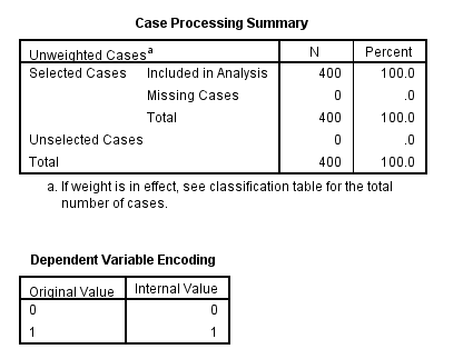
The first table above shows a breakdown of the number of cases used and not used in the analysis. The second table above gives the coding for the outcome variable, admit.

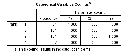
The table above shows how the values of the categorical variable rank were handled, there are terms (essentially dummy variables) in the model for rank=1,rank=2, and rank=3; rank=4 is the omitted category.

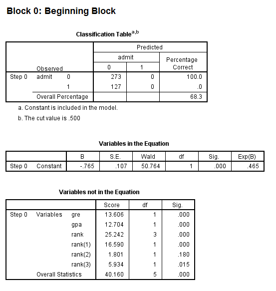
The first model in the output is a null model, that is, a model with no predictors.
The constant in the table labeled Variables in the Equation gives the unconditional log odds of admission (i.e., admit=1).
The table labeled Variables not in the Equation gives the results of a score test, also known as a Lagrange multiplier test. The column labeled Score gives the estimated change in model fit if the term is added to the model, the other two columns give the degrees of freedom, and p-value (labeled Sig.) for the estimated change. Based on the table above, all three of the predictors, gre, gpa, and rank, are expected to improve the fit of the model.

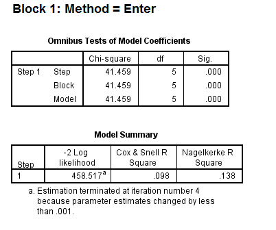
The first table above gives the overall test for the model that includes the predictors. The chi-square value of 41.46 with a p-value of less than 0.0005 tells us that our model as a whole fits significantly better than an empty model (i.e., a model with no predictors).
The -2*log likelihood (458.517) in the Model Summary table can be used in comparisons of nested models, but we won’t show an example of that here. This table also gives two measures of pseudo R-square.

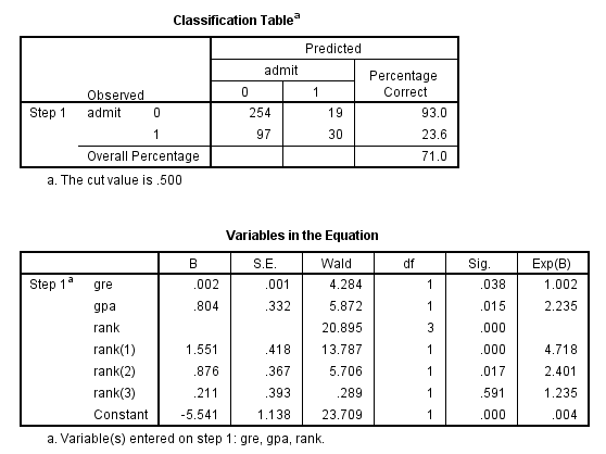
In the table labeled Variables in the Equation we see the coefficients, their standard errors, the Wald test statistic with associated degrees of freedom and p-values, and the exponentiated coefficient (also known as an odds ratio). Both gre and gpa are statistically significant. The overall (i.e., multiple degree of freedom) test for rank is given first, followed by the terms for rank=1, rank=2, and rank=3. The overall effect of rank is statistically significant, as are the terms for rank=1 and rank=2. The logistic regression coefficients give the change in the log odds of the outcome for a one unit increase in the predictor variable.
- For every one unit change in gre, the log odds of admission (versus non-admission) increases by 0.002.
- For a one unit increase in gpa, the log odds of being admitted to graduate school increases by 0.804.
- The indicator variables for rank have a slightly different interpretation. For example, having attended an undergraduate institution with rank of 1, versus an institution with a rank of 4, increases the log odds of admission by 1.551.

Things to consider

Empty cells or small cells: You should check for empty or small

cells by doing a crosstab between categorical predictors and the outcome variable. If a cell has very few cases (a small cell), the model may become unstable or it might not run at all.
Separation or quasi-separation (also called perfect prediction), a condition in which the outcome does not vary at some levels of the independent variables. See our page FAQ: What is complete or quasi-complete separation in logistic/probit regression and how do we deal with them? for information on models with perfect prediction.
Sample size: Both logit and probit models require more cases than OLS regression because they use maximum likelihood estimation techniques. It is also important to keep in mind that when the outcome is rare, even if the overall dataset is large, it can be difficult to estimate a logit model.
Pseudo-R-squared: Many different measures of pseudo-R-squared exist. They all attempt to provide information similar to that provided by R-squared in OLS regression; however, none of them can be interpreted exactly as R-squared in OLS regression is interpreted. For a discussion of various pseudo-R-squareds see Long and Freese (2006) or our FAQ page What are pseudo R-squareds?
Diagnostics: The diagnostics for logistic regression are different from those for OLS regression. For a discussion of model diagnostics for logistic regression, see Hosmer and Lemeshow (2000, Chapter 5). Note that diagnostics done for logistic regression are similar to those done for probit regression.

References

Hosmer, D. & Lemeshow, S. (2000). Applied Logistic Regression (Second Edition).

New York: John Wiley & Sons, Inc.
Long, J. Scott (1997). Regression Models for Categorical and Limited Dependent Variables.
Thousand Oaks, CA: Sage Publications.