使用Python scikit-learn 库实现神经网络算法

1：神经网络算法简介

2：Backpropagation算法详细介绍

3：非线性转化方程举例

4：自己实现神经网络算法NeuralNetwork

5：基于NeuralNetwork的XOR实例

6：基于NeuralNetwork的手写数字识别实例

7：scikit-learn中BernoulliRBM使用实例

8：scikit-learn中的手写数字识别实例

一：神经网络算法简介

1：背景

以人脑神经网络为启发，历史上出现过很多版本，但最著名的是backpropagation

2：多层向前神经网络（Multilayer  Feed-Forward Neural Network）

多层向前神经网络组成部分

输入层（input layer），隐藏层（hiddenlayer），输出层（output layer）

   每层由单元（units）组成

   输入层（input layer）是由训练集的实例特征向量传入

   经过连接结点的权重（weight）传入下一层，一层的输出是下一层的输入

   隐藏层的个数是任意的，输出层和输入层只有一个

   每个单元（unit）也可以被称作神经结点，根据生物学来源定义

   上图称为2层的神经网络（输入层不算）

   一层中加权的求和，然后根据非线性的方程转化输出

   作为多层向前神经网络，理论上，如果有足够多的隐藏层（hidden layers）和足够大的训练集，可以模拟出任何方程

 

3：设计神经网络结构

    3.1使用神经网络训练数据之前，必须确定神经网络层数，以及每层单元个数

    3.2特征向量在被传入输入层时通常被先标准化（normalize）和0和1之间（为了加强学习过程）

    3.3离散型变量可以被编码成每一个输入单元对应一个特征可能赋的值

        比如：特征值A可能取三个值（a0,a1,a2），可以使用三个输入单元来代表A

                    如果A=a0,那么代表a0的单元值就取1，其他取0

                    如果A=a1,那么代表a1的单元值就取1，其他取0，以此类推

    3.4神经网络即可以用来做分类（classification）问题，也可以解决回归（regression）问题

         3.4.1对于分类问题，如果是2类，可以用一个输入单元表示（0和1分别代表2类）

                                         如果多于两类，每一个类别用一个输出单元表示

                所以输入层的单元数量通常等于类别的数量 

        3.4.2没有明确的规则来设计最好有多少个隐藏层

               3.4.2.1根据实验测试和误差，以及准确度来实验并改进

4：算法验证——交叉验证法（Cross- Validation）

 

解读： 有一组输入集A,B，可以分成三组，第一次以第一组为训练集，求出一个准确度，第二次以第二组作为训练集，求出一个准确度，求出准确度，第三次以第三组作为训练集，求出一个准确度，然后对三个准确度求平均值

二：Backpropagation算法详细介绍

1：通过迭代性来处理训练集中的实例

2：输入层输入数

经过权重计算得到第一层的数据，第一层的数据作为第二层的输入，再次经过权重计算得到结果，结果和真实值之间是存在误差的，然后根据误差，反向的更新每两个连接之间的权重

3：算法详细介绍

输入：D : 数据集，| 学习率（learning rate），一个多层前向神经网络

    输出：一个训练好的神经网络（a trained neural network）

    3.1初始化权重（weights）和偏向（bias）：随机初始化在-1到1之间，或者-0.5到0.5之间，每个单元有一个偏向

    3.2对于每一个训练实例X，执行以下步骤：

         3.2.1：由输入层向前传送,输入->输出对应的计算为：

                              

                                         

                   计算得到一个数据，经过f 函数转化作为下一层的输入，f函数为：

          3.2.2：根据误差（error）反向传送

                     对于输出层（误差计算）：  Tj：真实值，Qj表示预测值

 

                     对于隐藏层（误差计算）：  Errk 表示前一层的误差， Wjk表示前一层与当前点的连接权重

                       

                     权重更新：  l：指学习比率（变化率），手工指定，优化方法是，随着数据的迭代逐渐减小

 

                     偏向更新：  l：同上

       3.3：终止条件

           3.3.1权重的更新低于某个阀值

           3.3.2预测的错误率低于某个阀值

           3.3.3达到预设一定的循环次数

4：结合实例讲解算法

0.9对用的是L，学习率

测试代码如下：

1.NeutralNetwork.py文件代码

#coding:utf-8

import numpy as np

#定义双曲函数和他们的导数
def tanh(x):
    return np.tanh(x)

def tanh_deriv(x):
    return 1.0 - np.tanh(x)**2

def logistic(x):
    return 1/(1 + np.exp(-x))

def logistic_derivative(x):
    return logistic(x)*(1-logistic(x))

#定义NeuralNetwork 神经网络算法
class NeuralNetwork:
    #初始化，layes表示的是一个list，eg[10,10,3]表示第一层10个神经元，第二层10个神经元，第三层3个神经元
    def __init__(self, layers, activation='tanh'):
        """
        :param layers: A list containing the number of units in each layer.
        Should be at least two values
        :param activation: The activation function to be used. Can be
        "logistic" or "tanh"
        """
        if activation == 'logistic':
            self.activation = logistic
            self.activation_deriv = logistic_derivative
        elif activation == 'tanh':
            self.activation = tanh
            self.activation_deriv = tanh_deriv

        self.weights = []
        #循环从1开始，相当于以第二层为基准，进行权重的初始化
        for i in range(1, len(layers) - 1):
            #对当前神经节点的前驱赋值
            self.weights.append((2*np.random.random((layers[i - 1] + 1, layers[i] + 1))-1)*0.25)
            #对当前神经节点的后继赋值
            self.weights.append((2*np.random.random((layers[i] + 1, layers[i + 1]))-1)*0.25)

            #训练函数   ，X矩阵，每行是一个实例 ，y是每个实例对应的结果，learning_rate 学习率，
    # epochs，表示抽样的方法对神经网络进行更新的最大次数
    def fit(self, X, y, learning_rate=0.2, epochs=10000):
        X = np.atleast_2d(X) #确定X至少是二维的数据
        temp = np.ones([X.shape[0], X.shape[1]+1]) #初始化矩阵
        temp[:, 0:-1] = X  # adding the bias unit to the input layer
        X = temp
        y = np.array(y) #把list转换成array的形式

        for k in range(epochs):
            #随机选取一行，对神经网络进行更新
            i = np.random.randint(X.shape[0])
            a = [X[i]]

            #完成所有正向的更新
            for l in range(len(self.weights)):
                a.append(self.activation(np.dot(a[l], self.weights[l])))
                #
            error = y[i] - a[-1]
            deltas = [error * self.activation_deriv(a[-1])]

            #开始反向计算误差，更新权重
            for l in range(len(a) - 2, 0, -1): # we need to begin at the second to last layer
                deltas.append(deltas[-1].dot(self.weights[l].T)*self.activation_deriv(a[l]))
            deltas.reverse()
            for i in range(len(self.weights)):
                layer = np.atleast_2d(a[i])
                delta = np.atleast_2d(deltas[i])
                self.weights[i] += learning_rate * layer.T.dot(delta)

                #预测函数
    def predict(self, x):
        x = np.array(x)
        temp = np.ones(x.shape[0]+1)
        temp[0:-1] = x
        a = temp
        for l in range(0, len(self.weights)):
            a = self.activation(np.dot(a, self.weights[l]))
        return a

2、测试代码

#coding:utf-8
'''
#基于NeuralNetwork的XOR（异或）示例
import numpy as np
from NeuralNetwork import NeuralNetwork

nn = NeuralNetwork([2,2,1], 'tanh')
X = np.array([[0, 0], [0, 1], [1, 0], [1, 1]])
y = np.array([0, 1, 1, 0])
nn.fit(X, y)
for i in [[0, 0], [0, 1], [1, 0], [1,1]]:
    print(i,nn.predict(i))
'''
'''
#基于NeuralNetwork的手写数字识别示例
import numpy as np
from sklearn.datasets import load_digits
from sklearn.metrics import confusion_matrix,classification_report
from sklearn.preprocessing import LabelBinarizer
from sklearn.cross_validation import train_test_split
from NeuralNetwork import NeuralNetwork

digits = load_digits()
X = digits.data
y = digits.target
X -= X.min()
X /= X.max()

nn =NeuralNetwork([64,100,10],'logistic')
X_train, X_test, y_train, y_test = train_test_split(X, y)
labels_train = LabelBinarizer().fit_transform(y_train)
labels_test = LabelBinarizer().fit_transform(y_test)
print "start fitting"
nn.fit(X_train,labels_train,epochs=3000)
predictions = []
for i in range(X_test.shape[0]):
    o = nn.predict(X_test[i])
    predictions.append(np.argmax(o))
print confusion_matrix(y_test, predictions)
print classification_report(y_test, predictions)
'''

#scikit-learn中的手写数字识别实例
import numpy as np
import matplotlib.pyplot as plt

from scipy.ndimage import convolve
from sklearn import linear_model, datasets, metrics
from sklearn.cross_validation import train_test_split
from sklearn.neural_network import BernoulliRBM
from sklearn.pipeline import Pipeline

###############################################################################
# Setting up

def nudge_dataset(X, Y):

    direction_vectors = [
        [[0, 1, 0],
         [0, 0, 0],
         [0, 0, 0]],

        [[0, 0, 0],
         [1, 0, 0],
         [0, 0, 0]],

        [[0, 0, 0],
         [0, 0, 1],
         [0, 0, 0]],

        [[0, 0, 0],
         [0, 0, 0],
         [0, 1, 0]]]

    shift = lambda x, w: convolve(x.reshape((8, 8)), mode='constant',
                                  weights=w).ravel()
    X = np.concatenate([X] +
                       [np.apply_along_axis(shift, 1, X, vector)
                        for vector in direction_vectors])
    Y = np.concatenate([Y for _ in range(5)], axis=0)
    return X, Y

# Load Data
digits = datasets.load_digits()
X = np.asarray(digits.data, 'float32')
X, Y = nudge_dataset(X, digits.target)
X = (X - np.min(X, 0)) / (np.max(X, 0) + 0.0001)  # 0-1 scaling

X_train, X_test, Y_train, Y_test = train_test_split(X, Y,
                                                    test_size=0.2,
                                                    random_state=0)

# Models we will use
logistic = linear_model.LogisticRegression()
rbm = BernoulliRBM(random_state=0, verbose=True)

classifier = Pipeline(steps=[('rbm', rbm), ('logistic', logistic)])

###############################################################################
# Training

# Hyper-parameters. These were set by cross-validation,
# using a GridSearchCV. Here we are not performing cross-validation to
# save time.
rbm.learning_rate = 0.06
rbm.n_iter = 20
# More components tend to give better prediction performance, but larger
# fitting time
rbm.n_components = 100
logistic.C = 6000.0

# Training RBM-Logistic Pipeline
classifier.fit(X_train, Y_train)

# Training Logistic regression
logistic_classifier = linear_model.LogisticRegression(C=100.0)
logistic_classifier.fit(X_train, Y_train)

###############################################################################
# Evaluation

print()
print("Logistic regression using RBM features:\n%s\n" % (
    metrics.classification_report(
        Y_test,
        classifier.predict(X_test))))

print("Logistic regression using raw pixel features:\n%s\n" % (
    metrics.classification_report(
        Y_test,
        logistic_classifier.predict(X_test))))

###############################################################################
# Plotting

plt.figure(figsize=(4.2, 4))
for i, comp in enumerate(rbm.components_):
    plt.subplot(10, 10, i + 1)
    plt.imshow(comp.reshape((8, 8)), cmap=plt.cm.gray_r,
               interpolation='nearest')
    plt.xticks(())
    plt.yticks(())
plt.suptitle('100 components extracted by RBM', fontsize=16)
plt.subplots_adjust(0.08, 0.02, 0.92, 0.85, 0.08, 0.23)

plt.show()

'''
from sklearn.neural_network import BernoulliRBM
X = [[0,0],[1,1]]
y = [0,1]
clf = BernoulliRBM().fit(X,y)
print

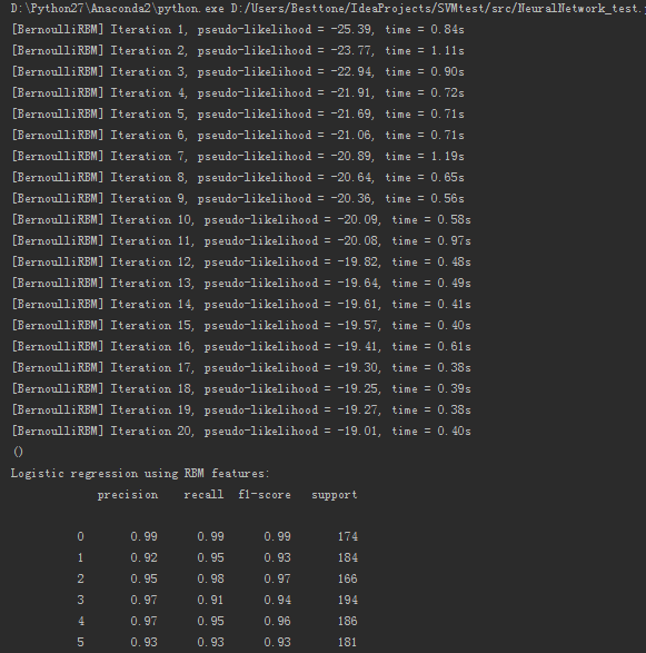
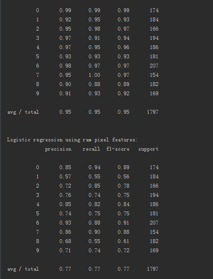
测试结果如下：