【转】Gabor 入门

Computer Vision Tutorials

Search

Primary Menu Skip to content

• Tutorials

Search for:  

Gabor Filters : A Practical Overview

April 27, 2014 krishnamurthyj 5 Comments

In this tutorial, we shall discuss Gabor filters, a classic technique, from a practical perspective.

Do not panic on seeing the equation that follows. It has been included here as a mere formality.

In the realms of image processing and computer vision, Gabor filters are generally used in texture analysis, edge detection, feature extraction, disparity estimation (in stereo vision), etc. Gabor filters are special classes of bandpass filters, i.e., they allow a certain ‘band’ of frequencies and reject the others.

In the course of this tutorial, we shall first discuss the essential results that we obtain when Gabor filters are applied on images. Then we move on to discuss the different parameters that control the output of the filter. This tutorial is aimed at delivering a practical overview of Gabor filters; hence, theoretical treatment is omitted (a tutorial that provides the essential theoretical rigor is currently in the pipeline).

At each stage of the discussion, results of relevant filters have been displayed. The implementation, though contained in the tutorial itself, draws heavily from the Python script that comes along with OpenCV. It has been simplified further so that it is simple for the beginners to work with.

To start with, Gabor filters are applied to images pretty much the same way as are conventional filters. We have a mask (a more precise (cooler) term for it would be ‘convolution kernel’) that represents the filter. By a mask, we mean to say that we have an array (usually a 2D array since 2D images are involved) of pixels in which each pixel is assigned a value (call it a ‘weight’). This array is slid over every pixel of the image and a convolution operation is performed (you can refer to the following link for more information on how a mask is applied to an image. http://en.wikipedia.org/wiki/Kernel_(image_processing) ).

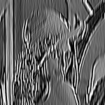
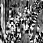
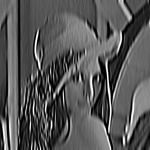
When a Gabor filter is applied to an image, it gives the highest response at edges and at points where texture changes. The following images show a test image and its transformation after the filter is applied.

Sample input to the Gabor filter

Output of the Gabor filter

A Gabor filter responds to edges and texture changes. When we say that a filter responds to a particular feature, we mean that the filter has a distinguishing value at the spatial location of that feature (when we’re dealing with applying convolution kernels in spatial domain, that is. The same holds for other domains, such as frequency domains, as well).

There are certain parameters that affect the output of a Gabor filter. In OpenCV Python, following is the structure of the function that is used to create a Gabor kernel.

cv2.getGaborKernel(ksize, sigma, theta, lambda, gamma, psi, ktype)

Each parameter is described very briefly in the OpenCV docs ( http://docs.opencv.org/trunk/modules/imgproc/doc/filtering.html ). Here’s a brief introduction to each of these parameters.

ksize is the size of the Gabor kernel. If ksize = (a, b), we then have a Gabor kernel of size a x b pixels. As with many other convolution kernels, ksize is preferably odd and the kernel is a square (just for the sake of uniformity).

sigma is the standard deviation of the Gaussian function used in the Gabor filter.

theta is the orientation of the normal to the parallel stripes of the Gabor function.

lambda is the wavelength of the sinusoidal factor in the above equation.

gamma is the spatial aspect ratio.

psi is the phase offset.

ktype indicates the type and range of values that each pixel in the Gabor kernel can hold.

Now that we’ve got a quaint feel of what each parameter means, let us delve deeper and understand the practical implication of the variation of each of these parameters.

The Code

This is a simplified version of gabor_threads.py, which is available in the OpenCV Python library. ( https://github.com/Itseez/opencv/blob/master/samples/python2/gabor_threads.py )

#!/usr/bin/env python

import numpy as np
import cv2

def build_filters():
 filters = []
 ksize = 31
 for theta in np.arange(0, np.pi, np.pi / 16):
 kern = cv2.getGaborKernel((ksize, ksize), 4.0, theta, 10.0, 0.5, 0, ktype=cv2.CV_32F)
 kern /= 1.5*kern.sum()
 filters.append(kern)
 return filters

def process(img, filters):
 accum = np.zeros_like(img)
 for kern in filters:
 fimg = cv2.filter2D(img, cv2.CV_8UC3, kern)
 np.maximum(accum, fimg, accum)
 return accum

if __name__ == '__main__':
 import sys

 print __doc__
 try:
 img_fn = sys.argv[1]
 except:
 img_fn = 'test.png'

 img = cv2.imread(img_fn)
 if img is None:
 print 'Failed to load image file:', img_fn
 sys.exit(1)

 filters = build_filters()

 res1 = process(img, filters)
 cv2.imshow('result', res1)
 cv2.waitKey(0)
 cv2.destroyAllWindows()

ksize

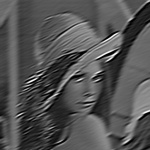
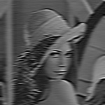
On varying ksize, the size of the convolution kernel varies. In the code above we modify the parameter ksize, while keeping the kernel square and of an odd size. We observe that there is no effect of the size of the convolution kernel on the output image. This also implies that the convolution kernel is scale invariant, since scaling the kernel’s size is analogous to scaling the size of the image. Here are a few results with varying ksize. For all the following images, sigma = 4.0, theta = 0, lambd = 10.0, gamma = 0.5, psi = 0, and ktype = cv2.CV_32F (i.e., each pixel of the convolution kernel holds a weight which is a 32-bit floating point number).

Input Image

ksize = 31 x 31

ksize = 51 x 51

ksize = 151 x 151

ksize = 531 x 531

(Roll over the images to view more information about each of them).

sigma

This parameter controls the width of the Gaussian envelope used in the Gabor kernel. Here are a few results obtained by varying this parameter.

sigma = 2

sigma = 3

sigma = 4

sigma = 5

sigma = 6

theta

This is perhaps one of the most important parameters of the Gabor filter. This parameter decides what kind of features the filter responds to. For example, giving theta a value of zero means that the filter is responsive only to horizontal features only. So, in order to obtain features at various angles in an image, we divide the interval between 0 and 180 into 16 equal parts, and compute a Gabor kernel for each value of theta thus obtained. Note that we’ve chosen 16 just because it was the default value in the OpenCV implementation. These parameter values could be modified to suit specific purposes. Following are the results of varying theta on the above input image.

theta = 11.25

theta = 22.5

theta = 33.75

theta = 45

theta = 56.25

theta = 67.5

theta = 78.75

theta = 90

theta = 101.25

theta = 112.5

theta = 123.75

theta = 135

theta = 146.25

theta = 157.5

theta = 168.75

theta = 180

lambda

Here’s the variation with lambda (theta is set to zero).

lambda = 8

lambda = 9

lambda = 10

lambda = 11

lambda = 12

gamma

Gamma controls the ellipticity of the gaussian. When gamma = 1, the gaussian envelope is circular.

gamma = 0.3

gamma = 0.4

gamma = 0.5

gamma = 0.6

gamma = 0.7

gamma = 1.0

psi

This parameter controls the phase offset.

psi = 0

psi = 10

psi = 50

psi = 90

So, we’ve examined the observable effects of various parameters on the output of the Gabor filter. Hope this tutorial helped. Will be back with more of such tuts soon.

About these ads

原文地址：https://cvtuts.wordpress.com/2014/04/27/gabor-filters-a-practical-overview/