Matlab周期图法使用FFT实现
参考文章:http://www.cnblogs.com/adgk07/p/9314892.html
首先根据他这个代码和我之前手上已经拥有的那个代码,编写了一个适合自己的代码。
首先模仿他的代码,测试成功。
思路:
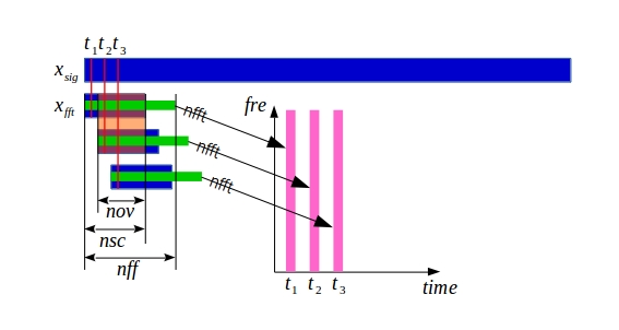
短时傅里叶变换,其实还是傅里叶变换,只不过把一段长信号按信号长度(nsc)、重叠点数(nov)重新采样。
% 结合之前两个版本的stft,实现自己的周期图法,力求通俗易懂,代码分明。
% 该代码写的时候是按照输入信号为实数的思路写的,在每个片段fft时进行前一半行的转置存储。后续代码思路已修改。

clear; clc; close all

% %---------------------Chirp 信号生成(start)---------------------

fa = [   ];                % 扫描频率上下限

fs = ;          % 采样频率

% 分辨率相关设定参数

te = ;             % [s] 扫频时间长度

fre = ;            % [s] 频率分辨率

tre = 0.002;        % [Hz] 时间分辨率

t = :/fs:te;                  % [s] 时间序列

sc = chirp(t,fa(),te,fa());   % 信号生成

%待传参(实参)

signal = sc;

nsc = floor(fs/fre);

nff = ^nextpow2(nsc);%每个窗口进行fft的长度

nov = floor(nsc*0.9);

% %---------------------Chirp 信号生成(end)---------------------

%% 使用fft实现周期图法

% Input

%       signal      - Signal vector         输入信号(行向量)

%       nsc         - Number SeCtion        每个小分段的信号长度

%       nov         - Number OverLap        重叠点数

%       fs          - Frequency of Sample   采样率

% Output

%       S           - A matrix that each colum is a FFT for time of nsc

%                    如果nfft为偶数,则S的行数为(nfft/+),如果nfft为奇数,则行数为(nfft+)/

%                    每一列是一个小窗口的FFT结果,因为matlab的FFT结果是对称的,只需要一半

%       W           - A vector labeling frequency

%       T           - A vector labeling time

% Signal Preprocessing

h = hamming(nsc, 'periodic');        % Hamming weight function  海明窗加权,窗口大小为nsc

L = length(signal);                  % Length of Signal         信号长度

nstep  = nsc-nov;                    % Number of STep per colum 每个窗口的步进

ncol   = fix( (L-nsc)/nstep ) + ;   % Number of CoLum          信号被分成了多少个片段

nfft   = ^nextpow2(nsc);            % Number of Fast Fourier Transformation  每个窗口FFT长度

nrow   = nfft/+;

%Symmetric results of FFT

STFT_X = zeros(nrow,ncol);  %STFT_X is a matrix,初始化最终结果

index=;%当前片段第一个信号位置在原始信号中的索引

for i=:ncol

    %提取当前片段信号值,并用海明窗进行加权(均为长度为nsc的行向量)

    temp_S=signal(index:index+nsc-).*h';

    %对长度为nsc的片段进行nfft点FFT变换

    temp_X=fft(temp_S,nfft);

    %从长度为nfft点(行向量)的fft变换中取一半(转换为列向量),存储到矩阵的列向量

    STFT_X(:,i)=temp_X(:nrow)';

    %将索引后移

    index=index + nstep;

end

 % Turn into DFT in dB

 STFT1 = abs(STFT_X/nfft);

 STFT1(:end-,:) = *STFT1(:end-,:);  % Add the value of the other half

 STFT3 = *log10(STFT1);                % Turn sound pressure into dB level

 % Axis Generating

 fax =(:(nfft/)) * fs/nfft;                        % Frequency axis setting

 tax = (nsc/ : nstep : nstep*(ncol-)+nsc/)/fs;    % Time axis generating

 [ffax,ttax] = meshgrid(tax,fax);                    % Generating grid of figure

 % Output

 W = ffax;

 T = ttax;

 S = STFT3;

 %% 画频谱图

 subplot(,,)                            % 绘制自编函数结果

 my_pcolor(W,T,S)

 caxis([-130.86,-13.667]);

 title('自编函数');

 xlabel('时间 second');

 ylabel('频率 Hz');

 subplot(,,)                            % 绘制 Matlab 函数结果

 s = spectrogram(signal,hamming(nsc),nov,nff,fs,'yaxis');

 % Turn into DFT in dB

 s1 = abs(s/nff);

 s2 = s1(:nff/+,:);             % Symmetric results of FFT

 s2(:end-,:) = *s2(:end-,:);  % Add the value of the other half

 s3 = *log10(s2);                % Turn sound pressure into dB level

 my_pcolor(W,T,s3 )

 caxis([-130.86,-13.667]);

 title('Matlab 自带函数');

 xlabel('时间 second');

 ylabel('频率 Hz');

 subplot(,,)                            % 两者误差

 my_pcolor(W,T,*log10(abs(.^(s3/)-.^(S/))))

 caxis([-,-13.667]);

 title('error');

 ylabel('频率 Hz');

 xlabel('时间 second');

 suptitle('Spectrogram 实现与比较');
内部调用了my_pcolor.m
function [  ] = my_pcolor( f , t , s )

%MY_PCOLOR 绘图函数

% Input

%       f               - 频率轴矩阵

%       t               - 时间轴矩阵

%       s               - 幅度轴矩阵

    gca = pcolor(f,t,s);                      % 绘制伪彩色图

        set(gca, 'LineStyle','none');         % 取消网格,避免一片黑

    handl = colorbar;                         % 彩图坐标尺

        set(handl, 'FontName', 'Times New Roman', 'FontSize', )

        ylabel(handl, 'Magnitude, dB')        % 坐标尺名称

end
接下来在主体不变的情况下,修改输入信号和函数返回结果,使其和自己之前的代码效果相同。
其实只要搞清楚了理论,实现上很简单。
一、首先分析Matlab周期图法API。
[spec_X,spec_f,spec_t]=spectrogram(signal,hamming(nsc, 'periodic'),nov,nff,Fs);
如果函数没有返回结果的调用,MATLAB直接帮我们绘图了。
1)当输入信号为复数时的代码:
clear

clc

close all

Fs = ;            % Sampling frequency

T = /Fs;             % Sampling period

L = ;             % Length of signal

t = (:L-)*T;        % Time vector

S = *sin(**pi*t)+*cos(**pi*t)*j;

nsc=;%海明窗的长度,即每个窗口的长度

nov=;%重叠率

nff= max(,^nextpow2(nsc));%N点采样长度

%% matlab自带函数

figure()

spectrogram(S,hamming(nsc, 'periodic'),nov,nff,Fs);

title('spectrogram函数画图')

[spec_X,spec_f,spec_t]=spectrogram(S,hamming(nsc, 'periodic'),nov,nff,Fs);
变量:

其中:
spec_X矩阵行数为nff,列数是根据信号signal的长度和每个片段nsc分割决定的,共计col列。
spec_f 为nff*1的列向量。
spec_t为 1*ncol的行向量。
此时自己实现的Matlab代码为:
 % 结合之前两个版本的stft,实现自己的周期图法,力求通俗易懂,代码分明。

 clear; clc; close all

 %% 信号输入基本参数

 Fs = ;            % Sampling frequency

 T = /Fs;             % Sampling period

 L = ;             % Length of signal

 t = (:L-)*T;        % Time vector

 S = *sin(**pi*t)+*cos(**pi*t)*j;

 %传参

 signal = S;

 nsc    = ;                     %每个窗口的长度,也即海明窗的长度

 nff    = max(,^nextpow2(nsc));%每个窗口进行fft的长度

 nov    = ;                       %重叠率

 fs     = Fs;                      %采样率

 %% 使用fft实现周期图法

 %后续可封装为函数:

 % function [ S , W , T ] = mf_spectrogram...

 %     ( signal , nsc , nov , fs )

 % Input

 %       signal      - Signal vector         输入信号(行向量)

 %       nsc         - Number SeCtion        每个小分段的信号长度

 %       nov         - Number OverLap        重叠点数

 %       fs          - Frequency of Sample   采样率

 % Output

 %       S           - A matrix that each colum is a FFT for time of nsc

 %                    如果nfft为偶数,则S的行数为(nfft/+),如果nfft为奇数,则行数为(nfft+)/

 %                    每一列是一个小窗口的FFT结果,因为matlab的FFT结果是对称的,只需要一半

 %       W           - A vector labeling frequency   频率轴

 %       T           - A vector labeling time        时间轴

 % Signal Preprocessing

 h = hamming(nsc, 'periodic');        % Hamming weight function  海明窗加权,窗口大小为nsc

 L = length(signal);                  % Length of Signal         信号长度

 nstep  = nsc-nov;                    % Number of STep per colum 每个窗口的步进

 ncol   = fix( (L-nsc)/nstep ) + ;   % Number of CoLum          信号被分成了多少个片段

 nfft   = max(,^nextpow2(nsc));   % Number of Fast Fourier Transformation  每个窗口FFT长度

 nrow   = nfft/+;

 %

 %

 STFT1 = zeros(nfft,ncol);  %STFT1 is a matrix 初始化最终结果

 index  = ;%当前片段第一个信号位置在原始信号中的索引

 for i=:ncol

     %提取当前片段信号值,并用海明窗进行加权(均为长度为nsc的行向量)

     temp_S=signal(index:index+nsc-).*h';

     %对长度为nsc的片段进行nfft点FFT变换

     temp_X=fft(temp_S,nfft);

     %将长度为nfft点(行向量)的fft变换转换为列向量,存储到矩阵的列向量

     STFT1(:,i)=temp_X';

     %将索引后移

     index=index + nstep;

 end

 %如果是为了和标准周期图法进行误差比较,则后续计算(abs,*,log(+1e-))不需要做,只需

 %plot(abs(spec_X)-abs(STFT1))比较即可

 STFT2 = abs(STFT1/nfft);

 %nfft是偶数,说明首尾是奈奎斯特点,只需对2:end-1的数据乘以2

 STFT2(:end-,:) = *STFT2(:end-,:);  % Add the value of the other half

 %STFT3 = *log10(STFT1);                % Turn sound pressure into dB level

 STFT3 = *log10(STFT2 + 1e-);          % convert amplitude spectrum to dB (min = - dB)

 % Axis Generating

 fax =(:(nfft-)) * fs./nfft;                        % Frequency axis setting

 tax = (nsc/ : nstep : nstep*(ncol-)+nsc/)/fs;     % Time axis generating

  % Output

  W = fax;

  T = tax;

  S = STFT3;

 %% matlab自带函数

 figure();

 spectrogram(signal,hamming(nsc, 'periodic'),nov,nff,Fs);

 title('spectrogram函数画图')

 [spec_X,spec_f,spec_t]=spectrogram(signal,hamming(nsc, 'periodic'),nov,nff,Fs);

 %减法,看看差距

 figure()

 plot(abs(spec_X)-abs(STFT1))

 %% 画频谱图

 figure

 %利用了SIFT3

 surf(W, T,  S')

 shading interp

 axis tight

 box on

 view(, )

 set(gca, 'FontName', 'Times New Roman', 'FontSize', )

 xlabel('Frequency, Hz')

 ylabel('Time, s')

 title('Amplitude spectrogram of the signal')

 handl = colorbar;

 set(handl, 'FontName', 'Times New Roman', 'FontSize', )

 ylabel(handl, 'Magnitude, dB')

 %跳频图

 figure();

 surf(T,W,S)

 shading interp

 axis tight

 box on

 view(, )

 set(gca, 'FontName', 'Times New Roman', 'FontSize', )

 ylabel('Frequency, Hz')

 xlabel('Time, s')

 title('Amplitude spectrogram of the signal')

 handl = colorbar;

 set(handl, 'FontName', 'Times New Roman', 'FontSize', )

 ylabel(handl, 'Magnitude, dB')
重点关注8行、59行、66行、69行、82行
其实此时只要牢牢记住结果集中行数为nfft就行了。
2)当输入信号为实数时的代码:
clear
clc
close all
Fs = 1000; % Sampling frequency
T = 1/Fs; % Sampling period
L = 1000; % Length of signal
t = (0:L-1)*T; % Time vector
S = 20*sin(150*2*pi*t)+40*cos(250*2*pi*t);
nsc=100;%海明窗的长度,即每个窗口的长度
nov=0;%重叠率
nff= max(256,2^nextpow2(nsc));%N点采样长度
%% matlab自带函数
figure(1)
spectrogram(S,hamming(nsc, 'periodic'),nov,nff,Fs);
title('spectrogram函数画图')
[spec_X,spec_f,spec_t]=spectrogram(S,hamming(nsc, 'periodic'),nov,nff,Fs);
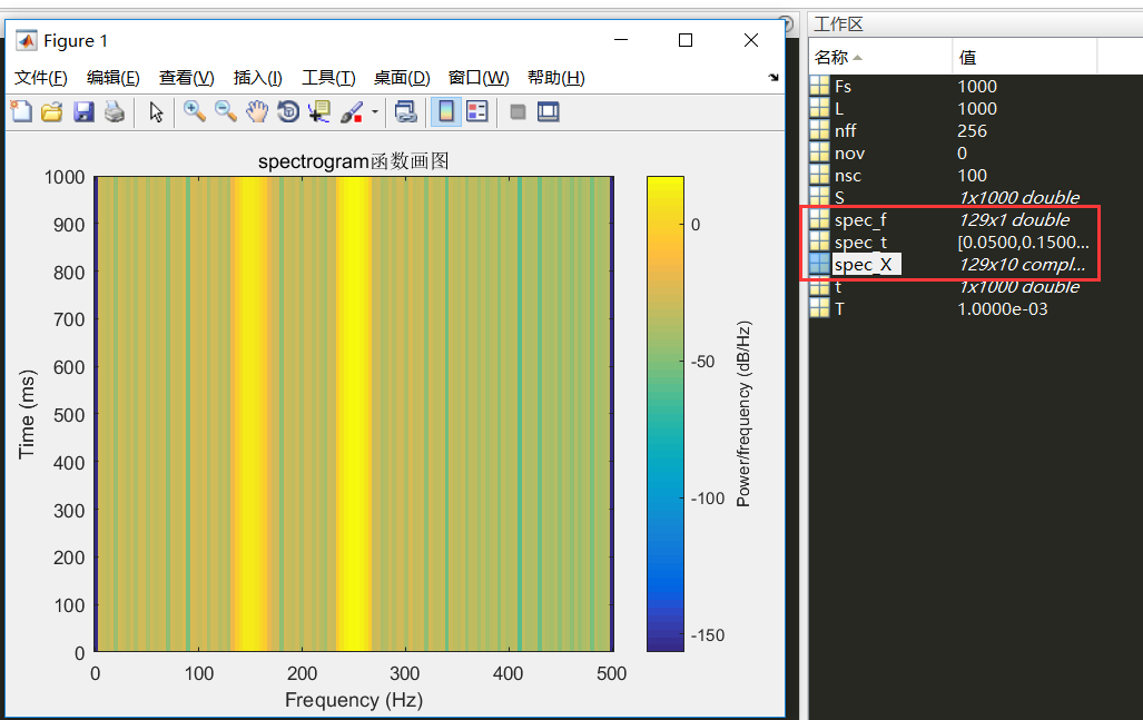
其中:
spec_X矩阵行数为nff/2+1,列数是根据信号signal的长度和每个片段nsc分割决定的,共计col列。
spec_f 为nff/2+1*1的列向量。
spec_t为 1*ncol的行向量。
主要是因为输入信号为实数时,fft变换的结果有一半是对称的,不必考虑。
自己实现的Matlab代码为:
 % 结合之前两个版本的stft,实现自己的周期图法,力求通俗易懂,代码分明。

 clear; clc; close all

 %% 信号输入基本参数

 Fs = ;            % Sampling frequency

 T = /Fs;             % Sampling period

 L = ;             % Length of signal

 t = (:L-)*T;        % Time vector

 S = *sin(**pi*t)+*cos(**pi*t);

 %传参

 signal = S;

 nsc    = ;                     %每个窗口的长度,也即海明窗的长度

 nff    = max(,^nextpow2(nsc));%每个窗口进行fft的长度

 nov    = ;                       %重叠率

 fs     = Fs;                      %采样率

 %% 使用fft实现周期图法

 %后续可封装为函数:

 % function [ S , W , T ] = mf_spectrogram...

 %     ( signal , nsc , nov , fs )

 % Input

 %       signal      - Signal vector         输入信号(行向量)

 %       nsc         - Number SeCtion        每个小分段的信号长度

 %       nov         - Number OverLap        重叠点数

 %       fs          - Frequency of Sample   采样率

 % Output

 %       S           - A matrix that each colum is a FFT for time of nsc

 %                    如果nfft为偶数,则S的行数为(nfft/+),如果nfft为奇数,则行数为(nfft+)/

 %                    每一列是一个小窗口的FFT结果,因为matlab的FFT结果是对称的,只需要一半

 %       W           - A vector labeling frequency   频率轴

 %       T           - A vector labeling time        时间轴

 % Signal Preprocessing

 h = hamming(nsc, 'periodic');        % Hamming weight function  海明窗加权,窗口大小为nsc

 L = length(signal);                  % Length of Signal         信号长度

 nstep  = nsc-nov;                    % Number of STep per colum 每个窗口的步进

 ncol   = fix( (L-nsc)/nstep ) + ;   % Number of CoLum          信号被分成了多少个片段

 nfft   = max(,^nextpow2(nsc));   % Number of Fast Fourier Transformation  每个窗口FFT长度

 nrow   = nfft/+;

 %

 %

 STFT1 = zeros(nfft,ncol);  %STFT1 is a matrix 初始化最终结果

 index  = ;%当前片段第一个信号位置在原始信号中的索引

 for i=:ncol

     %提取当前片段信号值,并用海明窗进行加权(均为长度为nsc的行向量)

     temp_S=signal(index:index+nsc-).*h';

     %对长度为nsc的片段进行nfft点FFT变换

     temp_X=fft(temp_S,nfft);

     %将长度为nfft点(行向量)的fft变换转换为列向量,存储到矩阵的列向量

     STFT1(:,i)=temp_X';

     %将索引后移

     index=index + nstep;

 end

 % -----当输入信号为实数时,对其的操作(也就是说只考虑信号的前一半)

 % 由于实数FFT的对称性,提取STFT1的nrow行

 STFT_X = STFT1(:nrow,:);             % Symmetric results of FFT

 %如果是为了和标准周期图法进行误差比较,则后续计算(abs,*,log(+1e-))不需要做,只需

 %plot(abs(spec_X)-abs(STFT_X))比较即可

 STFT2 = abs(STFT_X/nfft);

 %nfft是偶数,说明首尾是奈奎斯特点,只需对2:end-1的数据乘以2

 STFT2(:end-,:) = *STFT2(:end-,:);  % Add the value of the other half

 %STFT3 = *log10(STFT1);                % Turn sound pressure into dB level

 STFT3 = *log10(STFT2 + 1e-);          % convert amplitude spectrum to dB (min = - dB)

 % Axis Generating

 fax =(:(nrow-)) * fs./nfft;                        % Frequency axis setting

 tax = (nsc/ : nstep : nstep*(ncol-)+nsc/)/fs;     % Time axis generating

  % Output

  W = fax;

  T = tax;

  S = STFT3;

 %% matlab自带函数

 figure();

 spectrogram(signal,hamming(nsc, 'periodic'),nov,nff,Fs);

 title('spectrogram函数画图')

 [spec_X,spec_f,spec_t]=spectrogram(signal,hamming(nsc, 'periodic'),nov,nff,Fs);

 %减法,看看差距

 figure()

 plot(abs(spec_X)-abs(STFT_X))

 %% 画频谱图

 figure

 %利用了SIFT3

 surf(W, T,  S')

 shading interp

 axis tight

 box on

 view(, )

 set(gca, 'FontName', 'Times New Roman', 'FontSize', )

 xlabel('Frequency, Hz')

 ylabel('Time, s')

 title('Amplitude spectrogram of the signal')

 handl = colorbar;

 set(handl, 'FontName', 'Times New Roman', 'FontSize', )

 ylabel(handl, 'Magnitude, dB')

 %跳频图

 figure();

 surf(T,W,S)

 shading interp

 axis tight

 box on

 view(, )

 set(gca, 'FontName', 'Times New Roman', 'FontSize', )

 ylabel('Frequency, Hz')

 xlabel('Time, s')

 title('Amplitude spectrogram of the signal')

 handl = colorbar;

 set(handl, 'FontName', 'Times New Roman', 'FontSize', )

 ylabel(handl, 'Magnitude, dB')
主要记到行数为nrow=nfft/2+1行。
重点关注代码8行,57行,62行,85行。
二、分析思路
1)自己在使用fft实现时,通过一个for循环,对每个nsc长度的片段进行加窗、nfft点的fft变换。
2)
1. 当输入信号为实数时,由于fft的对称性,从结果SIFT1仅取fft结果行数的一半放到结果矩阵SIFT_X中去。
2. 当输入信号为复数时,该矩阵的行数仍然为nff行,因此结果集即为SIFT1。
3. 此时每一列即是一个小片段的fft变换的结果,该列结果是复数。 可以和Matlab API得到的结果进行差值比较,发现结果完全一样。
这3处分析的不同,也正是两个自己实现代码的修改处,可参考上述代码。
3)后续由于考虑到绘图、幅值、频谱的影响,因此又在复数矩阵的结果上进行了一些运算,因此在后续封装为函数时根据需要进行改进。
Matlab周期图法使用FFT实现的更多相关文章
- 基2时抽8点FFT的matlab实现流程及FFT的内部机理
前言 本来想用verilog描述FFT算法,虽然是8点的FFT算法,但写出来的资源用量及时延也不比调用FFT IP的好, 还是老实调IP吧,了解内部机理即可,无需重复发明轮子. 参考 https:// ...
- 【Matlab】快速傅里叶变换/ FFT/ fftshift/ fftshift(fft(fftshift(s)))
[自我理解] fft:可以指定点数的快速傅里叶变换 fftshift:将零频点移到频谱的中间 用法: Y=fftshift(X) Y=fftshift(X,dim) 描述:fftshift移动零频点到 ...
- MatLab实现FFT与功率谱
FFT和功率谱估计 用Fourier变换求取信号的功率谱---周期图法 clf; Fs=1000; N=256;Nfft=256;%数据的长度和FFT所用的数据长度 n=0:N-1;t=n/Fs;%采 ...
- FFT原理及C++与MATLAB混合编程详细介绍
一:FFT原理 1.1 DFT计算 在一个周期内的离散傅里叶级数(DFS)变换定义为离散傅里叶变换(DFT). \[\begin{cases} X(k) = \sum_{n=0}^{N-1}x(n)W ...
- C#实现FFT(递归法)
C#实现FFT(递归法) 1. C#实现复数类 我们在进行信号分析的时候,难免会使用到复数.但是遗憾的是,C#没有自带的复数类,以下提供了一种复数类的构建方法. 复数相比于实数,可以理解为一个二维数, ...
- MATLAB处理信号得到频谱、相谱、功率谱
(此帖引至网络资源,仅供参考学习)第一:频谱 一.调用方法 X=FFT(x):X=FFT(x,N):x=IFFT(X);x=IFFT(X,N) 用MATLAB进行谱分析时注意: (1)函数FFT返回值 ...
- 经典功率谱估计及Matlab仿真
原文出自:http://www.cnblogs.com/jacklu/p/5140913.html 功率谱估计在分析平稳各态遍历随机信号频率成分领域被广泛使用,并且已被成功应用到雷达信号处理.故障诊断 ...
- matlab 功率谱分析
matlab 功率谱分析 1.直接法:直接法又称周期图法,它是把随机序列x(n)的N个观测数据视为一能量有限的序列,直接计算x(n)的离散傅立叶变换,得X(k),然后再取其幅值的平方,并除以N,作为序 ...
- (转) 经典功率谱估计及Matlab仿真
原文出自:http://www.cnblogs.com/jacklu/p/5140913.html 功率谱估计在分析平稳各态遍历随机信号频率成分领域被广泛使用,并且已被成功应用到雷达信号处理.故障诊断 ...
随机推荐
- 冲刺One之站立会议1
接到任务之后的第一天,大家都分头查找了一些相关资料,目的是最终确定用什么语言编写程序.李琦负责对Java实现聊天室进行调研.郭婷和朱慧敏负责对C#进行调研.李敏和刘子晗负责对QT的实现进行调研.并讨论 ...
- beat冲刺(3/7)
目录 摘要 团队部分 个人部分 摘要 队名:小白吃 组长博客:hjj 作业博客:beta冲刺(3/7) 团队部分 后敬甲(组长) 过去两天完成了哪些任务 整理博客 ppt模板 接下来的计划 做好机动. ...
- OSI协议和TCP/IP协议笔记
1.OSI协议: 第7层应用层:OSI中的最高层.是用户与网络的接口.该层通过应用程序来完成网络用户的应用需求,如文件传输.收发电子邮件等.在此常见的协议有:HTTP,HTTPS,FTP,TELNET ...
- Centos7 虚拟机复制后网卡问题 Job for network.service failed
在运行“/etc/init.d/network restart”命令时,出现错误“Job for network.service failed. See 'systemctl status netwo ...
- python 菜鸟入门
python 菜鸟博客: http://www.cnblogs.com/wupeiqi/articles/5433893.html http://www.cnblogs.com/linhaifeng/ ...
- Webpack简易入门教程
<!-- 其实网上关于webpack的教程已经很多了,但是本人在学习过程中发现很多教程有错误,或者写的很不全面,结果做的过程出现各种各样的问题,对新手不但不友好还会让人浪费很多不必要的时间.所以 ...
- Mxnet Windows配置
MXNET Windows 编译安装(Python) 本文只记录Mxnet在windows下的编译安装,更多环境配置请移步官方文档:http://mxnet.readthedocs.io/en/lat ...
- NOIP赛前集训营-提高组(第一场)#A 中位数
题目描述 小N得到了一个非常神奇的序列A.这个序列长度为N,下标从1开始.A的一个子区间对应一个序列,可以由数对[l,r]表示,代表A[l], A[l + 1], ..., A[r]这段数.对于一 ...
- 【刷题】BZOJ 3262 [HNOI2008]GT考试
Description 阿申准备报名参加GT考试,准考证号为N位数X1X2....Xn(0<=Xi<=9),他不希望准考证号上出现不吉利的数字. 他的不吉利数学A1A2...Am(0< ...
- tarjan解决路径询问问题
好久没更新了,就更一篇普及组内容好了. 首先我们考虑如何用tarjan离线求出lca,伪代码大致如下: def tarjan(x): 将x标记为已访问 for c in x的孩子: tarjan(c) ...