Denoising Diffusion Probabilistic Models (DDPM)

概
主要内容
代码

Ho J., Jain A. and Abbeel P. Denoising diffusion probabilistic models. In Advances in Neural Information Processing Systems (NIPS), 2020.

[Page E. Approximating to the cumulative normal function and its inverse for use on a pocket calculator. Applied Statistics, vol. 26, pp. 75-76, 1977.]

Yerukala R., Boiroju N. K. Approximations to standard normal distribution function. Journal of Scientific and Engineering Research, vol. 6, pp. 515-518, 2015.

概

diffusion model和变分界的结合.

对抗鲁棒性上已经有多篇论文用DDPM生成的数据用于训练了, 可见其强大.

主要内容

Diffusion models

reverse process

从$p(x_T) = \mathcal{N}(x_T; 0, I)$出发:

\[p_{\theta}(x_{0:T}) := p(X_T) \prod_{t=1}^T p_{\theta}(x_{t-1}|x_t), \quad p_{\theta}(x_{t-1}|x_t) := \mathcal{N}(x_{t-1}; \mu_{\theta}(x_{t}, t), \Sigma_{\theta}(x_t, t)),
\]

注意这个过程我们拟合均值$\mu_{\theta}$和协方差矩阵$\Sigma_{\theta}$.

这部分的过程逐步将噪声'恢复'为图片(信号)$x_0$.

forward process

\[q(x_{1:T}|x_0) := \prod_{t=1}^{T}q(x_t|x_{t-1}), \quad q(x_t|x_{t-1}):= \mathcal{N}(x_t; \sqrt{1 - \beta_t} x_{t-1}, \beta_t I).
\]

其中$\beta_t$是可训练的参数或者人为给定的超参数.

这部分为将图片(信号)逐步添加噪声的过程.

变分界

对于参数$\theta$, 很自然地我们希望通过最小化其负对数似然来优化:

\[\begin{array}{ll}
\mathbb{E}_{p_{data}(x_0)} \bigg[-\log p_{\theta}(x_0) \bigg]
&=\mathbb{E}_{p_{data}(x_0)} \bigg[-\log \int p_{\theta}(x_{0:T}) \mathrm{d}x_{0:T} \bigg] \\
&=\mathbb{E}_{p_{data}(x_0)} \bigg[-\log \int q(x_{1:T}|x_0)\frac{p_{\theta}(x_{0:T})}{q(x_{1:T}|x_0)} \mathrm{d}x_{0:T} \bigg] \\
&=\mathbb{E}_{p_{data}(x_0)} \bigg[-\log \mathbb{E}_{q(x_{1:T}|x_0)} \frac{p_{\theta}(x_{0:T})}{q(x_{1:T}|x_0)} \bigg] \\
&\le -\mathbb{E}_{p_{data}(x_0)}\mathbb{E}_{q(x_{1:T}|x_0)} \bigg[\log \frac{p_{\theta}(x_{0:T})}{q(x_{1:T}|x_0)} \bigg] \\
&= -\mathbb{E}_q \bigg[\log \frac{p_{\theta}(x_{0:T})}{q(x_{1:T}|x_0)} \bigg] \\
&= -\mathbb{E}_q \bigg[\log p(x_T) + \sum_{t=1}^T \log \frac{p_{\theta}(x_{t-1}|x_t)}{q(x_t|x_{t-1})} \bigg] \\
&= -\mathbb{E}_q \bigg[\log p(x_T) + \sum_{t=2}^T \log \frac{p_{\theta}(x_{t-1}|x_t)}{q(x_t|x_{t-1})} + \log \frac{p_{\theta}(x_0|x_1)}{q(x_1|x_0)} \bigg] \\
&= -\mathbb{E}_q \bigg[\log p(x_T) + \sum_{t=2}^T \log \frac{p_{\theta}(x_{t-1}|x_t)}{q(x_{t-1}|x_t, x_0)} \cdot \frac{q(x_{t-1}|x_0)}{q(x_t|x_0)} + \log \frac{p_{\theta}(x_0|x_1)}{q(x_1|x_0)} \bigg] \\
&= -\mathbb{E}_q \bigg[\log \frac{p(x_T)}{q(x_T|x_0)} + \sum_{t=2}^T \log \frac{p_{\theta}(x_{t-1}|x_t)}{q(x_{t-1}|x_t, x_0)} + \log p_{\theta}(x_0|x_1) \bigg] \\
\end{array}
\]

注: $q=q(x_{1:T}|x_0)p_{data}(x_0)$, 下面另$q(x_0) := p_{data}(x_0)$.

又

\[\begin{array}{ll}
\mathbb{E}_q [\log \frac{q(x_T|x_0)}{p(x_T)}]
&= \int q(x_0, x_T) \log \frac{q(x_T|x_0)}{p(x_T)} \mathrm{d}x_0 \mathrm{d}x_T \\
&= \int q(x_0) q(x_T|x_0) \log \frac{q(x_T|x_0)}{p(x_T)} \mathrm{d}x_0 \mathrm{d}x_T \\
&= \int q(x_0) \mathrm{D_{KL}}(q(x_T|x_0) \| p(x_T)) \mathrm{d}x_0 \\
&= \int q(x_{0:T}) \mathrm{D_{KL}}(q(x'_T|x_0) \| p(x'_T)) \mathrm{d}x_{0:T} \\
&= \mathbb{E}_q \bigg[\mathrm{D_{KL}}(q(x'_T|x_0) \| p(x'_T)) \bigg].
\end{array}
\]

又

\[\begin{array}{ll}
\mathbb{E}_q [\log \frac{q(x_{t-1}|x_t, x_0)}{p_{\theta}(x_{t-1}|x_t)}]
&=\int q(x_0, x_{t-1}, x_t) \log \frac{q(x_{t-1}|x_t, x_0)}{p_{\theta}(x_{t-1}|x_t)} \mathrm{d}x_0 \mathrm{d}x_{t-1}\mathrm{d}x_t\\
&=\int q(x_0, x_t) \mathrm{D_{KL}}(q(x_{t-1}|x_t, x_0)\| p_{\theta}(x_{t-1}|x_t)) \mathrm{d}x_0 \mathrm{d}x_t\\
&=\mathbb{E}_q\bigg[\mathrm{D_{KL}}(q(x'_{t-1}|x_t, x_0)\| p_{\theta}(x'_{t-1}|x_t)) \bigg].
\end{array}
\]

故最后:

\[\mathcal{L} := \mathbb{E}_q \bigg[
\underbrace{\mathrm{D_{KL}}(q(x'_T|x_0) \| p(x'_T))}_{L_T} +
\sum_{t=2}^T \underbrace{\mathrm{D_{KL}}(q(x'_{t-1}|x_t, x_0)\| p_{\theta}(x'_{t-1}|x_t))}_{L_{t-1}}
\underbrace{-\log p_{\theta}(x_0|x_1)}_{L_0}.
\bigg]
\]

损失求解

因为无论forward, 还是 reverse process都是基于高斯分布的, 我们可以显示求解上面的各项损失:

首先, 对于forward process中的$x_t$:

\[\begin{array}{ll}
x_t
&= \sqrt{1 - \beta_t} x_{t-1} + \sqrt{\beta_t} \epsilon, \: \epsilon \sim \mathcal{N}(0, I) \\
&= \sqrt{1 - \beta_t} (\sqrt{1 - \beta_{t-1}} x_{t-2} + \sqrt{\beta_{t-1}} \epsilon') + \sqrt{\beta} \epsilon \\
&= \sqrt{1 - \beta_t}\sqrt{1 - \beta_{t-1}} x_{t-2} + \sqrt{1 - \beta_t}\sqrt{\beta_{t-1}} \epsilon' + \sqrt{\beta} \epsilon \\
&= \sqrt{1 - \beta_t}\sqrt{1 - \beta_{t-1}} x_{t-2} +
\sqrt{1 - (1 - \beta_t)(1 - \beta_{t-1})} \epsilon \\
&= \cdots \\
&= (\prod_{s=1}^t \sqrt{1 - \beta_s}) x_0 + \sqrt{1 - \prod_{s=1}^t (1 - \beta_s)} \epsilon,
\end{array}
\]

故

\[q(x_t|x_0) = \mathcal{N}(x_t|\sqrt{\bar{\alpha}_t}x_0, (1 - \bar{\alpha}_t)I), \: \bar{\alpha}_t := \prod_{s=1}^t \alpha_s, \alpha_s := 1 - \beta_s.
\]

对于后验分布$q(x_{t-1}|x_t, x_0)$, 我们有

\[\begin{array}{ll}
q(x_{t-1}|x_t, x_0)
&= \frac{q(x_t|x_{t-1})q(x_{t-1}|x_0)}{q(x_t|x_0)} \\
&\propto q(x_t|x_{t-1})q(x_{t-1}|x_0) \\
&\propto \exp\Bigg\{-\frac{1}{2 (1 - \bar{\alpha}_{t-1})\beta_t} \bigg[(1 - \bar{\alpha}_{t-1}) \|x_t - \sqrt{1 - \beta_t} x_{t-1}\|^2 + \beta_t \|x_{t-1} - \sqrt{\bar{\alpha}_{t-1}}x_0\|^2 \bigg]\Bigg\} \\
&\propto \exp\Bigg\{-\frac{1}{2 (1 - \bar{\alpha}_{t-1})\beta_t} \bigg[(1 - \bar{\alpha}_t)\|x_{t-1}\|^2 - 2(1 - \bar{\alpha}_{t-1}) \sqrt{\alpha_t} x_t^Tx_{t-1} - 2 \sqrt{\bar{\alpha}_{t-1}} \beta_t \bigg]\Bigg\} \\
\end{array}
\]

所以

\[q(x_{t-1}|x_t, x_0) \sim \mathcal{N}(x_{t-1}|\tilde{u}_t(x_t, x_0), \tilde{\beta}_t I),
\]

其中

\[\tilde{u}_t(x_t,x_0) := \frac{\sqrt{\bar{\alpha}_{t-1}}\beta_t}{1 - \bar{\alpha}_t} x_0 + \frac{\sqrt{\alpha_t}(1 - \bar{\alpha}_{t-1})}{1 - \bar{\alpha}_t} x_t,
\]

\[\tilde{\beta}_t = \frac{1 - \bar{\alpha}_{t-1}}{1 - \bar{\alpha}_t} \beta_t.
\]

$L_{t}$

$L_T$与$\theta$无关, 舍去.

作者假设$\Sigma_{\theta}(x_t, t) = \sigma_t^2 I$为非训练的参数, 其中

\[\sigma_t^2 = \beta_t | \tilde{\beta}_t,
\]

分别为$x_0 \sim \mathcal{N}(0, I)$和$x_0$为固定值时, 期望下KL散度的最优参数(作者说在实验中二者差不多).

故

\[L_{t} = \frac{1}{2 \sigma^2_t} \| \mu_{\theta}(x_t, t) - \tilde{u}_t(x_t, x_0)\|^2 +C, \quad t = 1,2,\cdots, T-1.
\]

又

\[x_t = \sqrt{\bar{\alpha}_t} x_0 + \sqrt{1 - \bar{\alpha}_t} \epsilon \Rightarrow x_0 = \frac{1}{\sqrt{\bar{\alpha}_t}}x_t - \frac{\sqrt{1 - \bar{\alpha}_t} }{\sqrt{\bar{\alpha}_t}} \epsilon.
\]

所以

\[\begin{array}{ll}
\mathbb{E}_q [L_{t-1} - C]
&= \mathbb{E}_{x_0, \epsilon} \bigg\{
\frac{1}{2 \sigma_t^2} \| \mu_{\theta}(x_t, t) - \tilde{u}_t\big( x_t, (\frac{1}{\sqrt{\bar{\alpha}_t}}x_t - \frac{\sqrt{1 - \bar{\alpha}_t} }{\sqrt{\bar{\alpha}_t}} \epsilon) \big)\|^2 \bigg\} \\
&= \mathbb{E}_{x_0, \epsilon} \bigg\{
\frac{1}{2 \sigma^2_t} \| \mu_{\theta}(x_t, t) -
\frac{1}{\sqrt{\alpha_t}} \big( x_t - \frac{\beta_t}{\sqrt{1 - \bar{\alpha}_t}} \epsilon \big) \bigg\} \\
\end{array}
\]

注: 上式子中$x_t$由$x_0, \epsilon$决定, 实际上$x_t = x_t(x_0, \epsilon)$, 故期望实际上是对$x_t$求期望.

既然如此, 我们不妨直接参数化$\mu_{\theta}$为

\[\mu_{\theta}(x_t, t):=
\frac{1}{\sqrt{\alpha_t}} \big( x_t - \frac{\beta_t}{\sqrt{1 - \bar{\alpha}_t}} \epsilon_{\theta}(x_t, t) \big),
\]

即直接建模残差$\epsilon$.

此时损失可简化为:

\[\mathbb{E}_{x_0, \epsilon} \bigg\{
\frac{\beta_t^2}{2\sigma_t^2 \alpha_t (1 - \bar{\alpha}_t)} \|\epsilon_{\theta}(\sqrt{\bar{\alpha}_t}x_0 + \sqrt{1 - \bar{\alpha}_t}\epsilon, t) - \epsilon\|^2
\bigg\}
\]

这个实际上时denoising score matching.

类似地, 从$p_{\theta}(x_{t-1}|x_t)$采样则为:

\[x_{t-1} =
\frac{1}{\sqrt{\alpha_t}} \big( x_t - \frac{\beta_t}{\sqrt{1 - \bar{\alpha}_t}} \epsilon_{\theta}(x_t, t) \big) + \sigma_t z, \: z \sim \mathcal{N}(0, I),
\]

这是Langevin dynamic的形式(步长和权重有点变化)

注: 这部分见here.

$L_0$

最后我们要处理$L_0$, 这里作者假设$x_0|x_1$满足一个离散分布, 首先图片取值于$\{0, 1, 2, \cdots, 255\}$, 并标准化至$[-1, 1]$. 假设

\[p_{\theta}(x_0|x_1) = \prod_{i=1}^D \int_{\delta_{-}(x_0^i)}^{\delta_+(x_0^i) } \mathcal{N}(x; \mu_{\theta}^i(x_1, 1), \sigma_1^2) \mathrm{d}x, \\
\delta_+(x) =
\left \{
\begin{array}{ll}
+\infty & \text{if } x = 1, \\
x + \frac{1}{255} & \text{if } x < 1.
\end{array}
\right .
\delta_- (x)
\left \{
\begin{array}{ll}
-\infty & \text{if } x = -1, \\
x - \frac{1}{255} & \text{if } x > -1.
\end{array}
\right .
\]

实际上就是将普通的正态分布划分为:

\[(-\infty, -1 + 1/255], (-1 + 1 / 255, -1 + 3/255], \cdots, (1 - 3/255, 1 - 1/255], (1 - 1 / 255, +\infty)
\]

各取值落在其中之一.

在实际代码编写中, 会遇到高斯函数密度函数估计的问题(直接求是做不到的), 作者选择用下列的估计方式:

\[\Phi(x) \approx \frac{1}{2} \Bigg\{1 + \tanh \bigg(\sqrt{2/\pi} (1 + 0.044715 x^2) \bigg) \Bigg\}.
\]

这样梯度也就能够回传了.

注: 该估计属于Page.

最后的算法

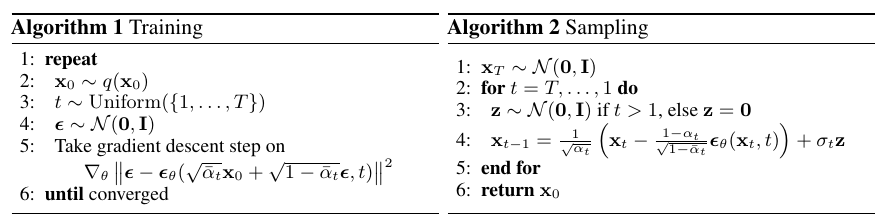
注: $t=1$对应$L_0$, $t=2,\cdots, T$对应$L_{1}, \cdots, L_{T-1}$.

注: 对于$L_t$作者省略了开始的系数, 这反而是一种加权.

作者在实际中是采样损失用以训练的.

细节

注意到, 作者的$\epsilon_{\theta}(\cdot, t)$是有显示强调$t$, 作者在实验中是通过attention中的位置编码实现的, 假设位置编码为$P$:

$ t = \text{Linear}(\text{ACT}(\text{Linear}(t * P)))$, 即通过两层的MLP来转换得到time_steps;
作者用的是U-Net结构, 在每个residual 模块中:

\[x += \text{Linear}(\text{ACT}(t)).
\]

参数	值
$T$	1000
$\beta_t$	$[0.0001, 0.02]$, 线性增长$1,2,\cdots, T$.
backbone	U-Net

注: 作者在实现中还用到了EMA等技巧.

代码

原文代码

lucidrains-denoising-diffusion-pytorch