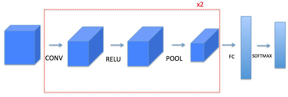
Convolutional Neural Network-week1编程题（一步步搭建CNN模型）

Convolutional Neural Networks: Step by Step

implement convolutional (CONV) and pooling (POOL) layers in numpy, including both forward propagation and (optionally) backward propagation.

Notation:

• Superscript \([l]\) denotes an object of the \(l^{th}\) layer.

  • Example: \(a^{[4]}\) is the \(4^{th}\) layer activation. \(W^{[5]}\) and \(b^{[5]}\) are the \(5^{th}\) layer parameters.

• Superscript \((i)\) denotes an object from the \(i^{th}\) example.

  • Example: \(x^{(i)}\) is the \(i^{th}\) training example input.

• Lowerscript \(i\) denotes the \(i^{th}\) entry of a vector.

  • Example: \(a^{[l]}_i\) denotes the \(i^{th}\) entry of the activations in layer \(l\), assuming this is a fully connected (FC) layer.

• \(n_H\), \(n_W\) and \(n_C\) denote respectively the height, width and number of channels of a given layer. If you want to reference a specific layer \(l\), you can also write \(n_H^{[l]}\), \(n_W^{[l]}\), \(n_C^{[l]}\).

• \(n_{H_{prev}}\), \(n_{W_{prev}}\) and \(n_{C_{prev}}\) denote respectively the height, width and number of channels of the previous layer. If referencing a specific layer \(l\), this could also be denoted \(n_H^{[l-1]}\), \(n_W^{[l-1]}\), \(n_C^{[l-1]}\).

1. Packages

import numpy as np
import h5py
import matplotlib.pyplot as plt

%matplotlib inline
plt.rcParams['figure.figsize'] = (5.0, 4.0) # set default size of plots
plt.rcParams['image.interpolation'] = 'nearest'
plt.rcParams['image.cmap'] = 'gray'

%load_ext autoreload
%autoreload 2

np.random.seed(1)

2. Outline of Assignment

• Convolution functions, including:

  • Zero Padding

  • Convolve window

  • Convolution forward

  • Convolution backward (optional)

• Pooling functions, including:

  • Pooling forward

  • Create mask

  • Distribute value

  • Pooling backward (optional)

Note: 每一步前向传播，都有对应的 反向传播，因此，你需要把每一步前向传播的parameters，存储到 cache中，用于反向传播.

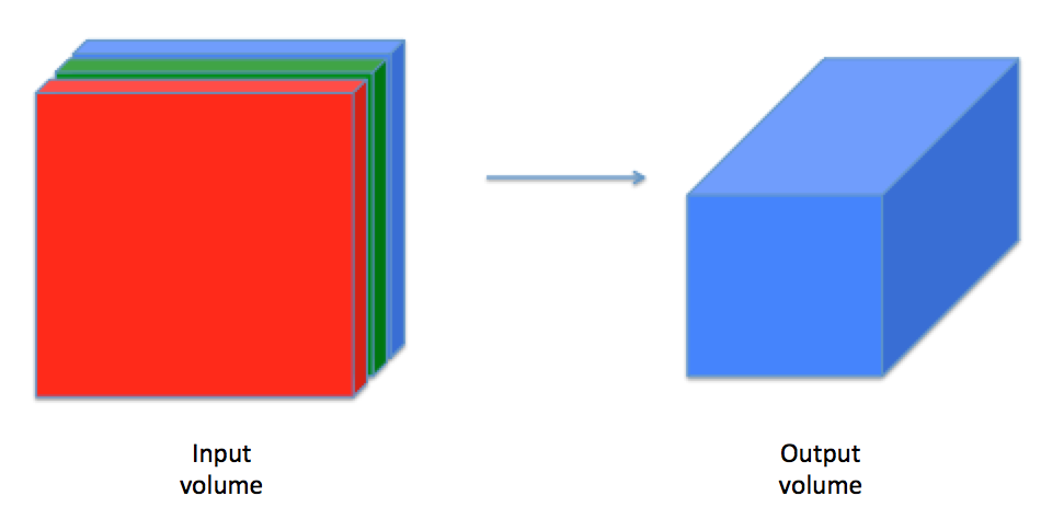
3. Convolutional Neural Networks

一个卷积层(convolutional layer)将一个输入量转换成不同大小的输出量，如图：

3.1 Zero-Padding

Zero-padding adds zeros around the border of an image:

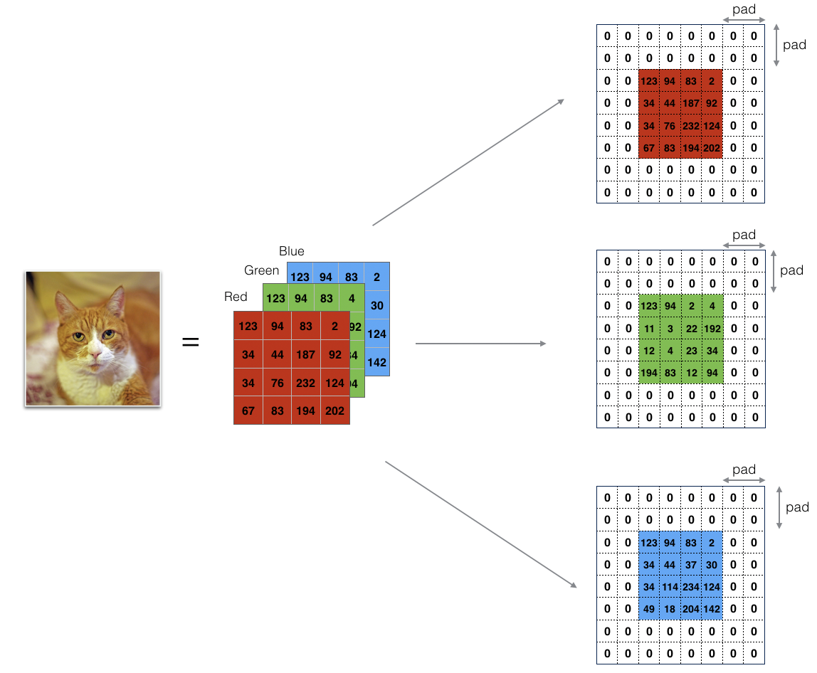
Figure 1 : Zero-Padding：Image (3 channels, RGB) with a padding of 2.

Zero-Padding的两个好处：

• 允许你使用 CONV layer 而不必要减小 the height and width of the volumes.(尤其是搭建深层网络时)(Same convolutions)

• 帮助我们保持图片边缘重要的信息. 没有Padding，很少有值，在下一层能够作为图片的边缘被像素值影响

Exercise:实现函数，用0填充一批示例X的所有图像. Note if you want to pad the array "a" of shape \((5,5,5,5,5)\) with pad = 1 for the 2nd dimension, pad = 3 for the 4th dimension and pad = 0 for the rest, you would do:

a = np.pad(a, ((0,0), (1,1), (0,0), (3,3), (0,0)), 'constant', constant_values = (..,..))

实现：

# GRADED FUNCTION: zero_pad

def zero_pad(X, pad):
    """
    Pad with zeros all images of the dataset X. The padding is applied to the height and width of an image,
    as illustrated in Figure 1.

    Argument:
    X -- python numpy array of shape (m, n_H, n_W, n_C) representing a batch of m images
    pad -- integer, amount of padding around each image on vertical and horizontal dimensions

    Returns:
    X_pad -- padded image of shape (m, n_H + 2*pad, n_W + 2*pad, n_C)
    """

    ### START CODE HERE ### (≈ 1 line)
    # X_pad: (m, n_H + 2*pad, n_W + 2*pad, n_C)
    X_pad = np.pad(X, ((0, 0), (pad, pad), (pad, pad), (0, 0)), 'constant', constant_values=0)
    ### END CODE HERE ###

    return X_pad

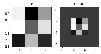
测试：

np.random.seed(1)
x = np.random.randn(4, 3, 3, 2)
x_pad = zero_pad(x, 2)
print ("x.shape =", x.shape)
print ("x_pad.shape =", x_pad.shape)
print ("x[1,1] =", x[1,1])
print ("x_pad[1,1] =", x_pad[1,1])

fig, axarr = plt.subplots(1, 2)
axarr[0].set_title('x')
axarr[0].imshow(x[0,:,:,0])
axarr[1].set_title('x_pad')
axarr[1].imshow(x_pad[0,:,:,0])

输出：

x.shape = (4, 3, 3, 2)

x_pad.shape = (4, 7, 7, 2)

x[1,1] = [[ 0.90085595 -0.68372786]

[-0.12289023 -0.93576943]

[-0.26788808 0.53035547]]

x_pad[1,1] = [[0. 0.]

[0. 0.]

[0. 0.]

[0. 0.]

[0. 0.]

[0. 0.]

[0. 0.]]

3.2 Single step of convolution

在这一部分中，实现一个卷积的步骤，在该步骤中，将过滤器应用到输入的单个位置中。这将构建卷积单元：

• 需要一个输入volume

• 将滤波器应用到输入的每个位置

• 输出一个不同大小的volume

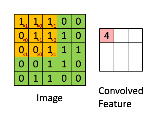
Figure 2 : Convolution operation 2x2的滤波器(filter) 和 步长(stride)为1 (stride = amount you move the window each time you slide)

计算机图像应用中，左边矩阵中的每个值对应于单个像素值，我们通过3x3滤波器与图像卷积，将其值元素与原始矩阵相乘，然后将它们求和并添加偏差。将实现一个卷积步骤，对应于将滤波器应用于其中一个位置以获得单个实值输出。

稍后将将此函数应用于输入的多个位置，以实现完全卷积操作。

Exercise：实现 conv_single_step().

# GRADED FUNCTION: conv_single_step

def conv_single_step(a_slice_prev, W, b):
    """
    Apply one filter defined by parameters W on a single slice (a_slice_prev) of the output activation
    of the previous layer.

    Arguments:
    a_slice_prev -- slice of input data of shape (f, f, n_C_prev)
    W -- Weight parameters contained in a window - matrix of shape (f, f, n_C_prev)
    b -- Bias parameters contained in a window - matrix of shape (1, 1, 1)

    Returns:
    Z -- a scalar value, result of convolving the sliding window (W, b) on a slice x of the input data
    """

    ### START CODE HERE ### (≈ 2 lines of code)
    # Element-wise product between a_slice and W. Do not add the bias yet.
    s = np.multiply(a_slice_prev, W)
    # Sum over all entries of the volume s.
    Z = np.sum(s)
    # Add bias b to Z. Cast b to a float() so that Z results in a scalar value.
    Z = Z + float(b)
    ### END CODE HERE ###

    return Z

测试：

np.random.seed(1)
a_slice_prev = np.random.randn(4, 4, 3)
W = np.random.randn(4, 4, 3)
b = np.random.randn(1, 1, 1)

Z = conv_single_step(a_slice_prev, W, b)
print("Z =", Z)

输出：

Z = -6.999089450680221

3.3 Convolutional Neural Networks - Forward pass

在前向传播中，你需要很多filters，并在输入上卷积，每次卷积，给你一个2D的矩阵输出，你将stack这些输出，组成一个3D volume：

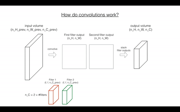
Exercise: 函数实现 在 input activation A_prev 上卷积filter W.

• A_prev作为输(上一层m inputs激活的输出). 由W表示F filters/weights，b表示bias vector

• 其中，每个filter都有自己的bias. 你可以访问包含 stride 和 padding的超参数字典

Hint:

1. 在matrix "a_prev"(shape(5,5,3))的左上角，选择一个2x2的slice，你需要: a_slice_prev = a_prev[0:2,0:2,:]

   • 你将使用 start/end indexes 定义 a_slice_prev

2. 要定义 a_slice，你需要首先定义他的corners： vert_start, vert_end, horiz_start and horiz_end，下图展示每个Corner如何用 h,w,f,s 定义：

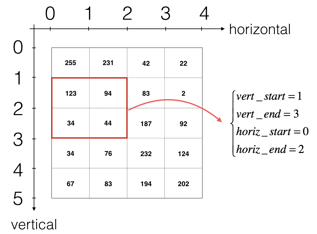
Figure 3 : Definition of a slice using vertical and horizontal start/end (with a 2x2 filter) (This figure shows only a single channel)

Reminder:

卷积后的shape与input shape 有关的公式:

\[n_H = \lfloor \frac{n_{H_{prev}} - f + 2 \times pad}{stride} \rfloor +1
\]

\[n_W = \lfloor \frac{n_{W_{prev}} - f + 2 \times pad}{stride} \rfloor +1
\]

\[n_C = \text{number of filters used in the convolution}
\]

使用for-loop实现：

# GRADED FUNCTION: conv_forward

def conv_forward(A_prev, W, b, hparameters):
    """
    Implements the forward propagation for a convolution function

    Arguments:
    A_prev -- output activations of the previous layer, numpy array of shape (m, n_H_prev, n_W_prev, n_C_prev)
    W -- Weights, numpy array of shape (f, f, n_C_prev, n_C)
    b -- Biases, numpy array of shape (1, 1, 1, n_C)
    hparameters -- python dictionary containing "stride" and "pad"

    Returns:
    Z -- conv output, numpy array of shape (m, n_H, n_W, n_C)
    cache -- cache of values needed for the conv_backward() function
    """

    ### START CODE HERE ###
    # Retrieve dimensions from A_prev's shape (≈1 line)
    (m, n_H_prev, n_W_prev, n_C_prev) = A_prev.shape

    # Retrieve dimensions from W's shape (≈1 line)
    (f, f, n_C_prev, n_C) = W.shape    # n_C: n_C个filter

    # Retrieve information from "hparameters" (≈2 lines)
    stride = hparameters['stride']
    pad = hparameters['pad']

    # Compute the dimensions of the CONV output volume using the formula given above. Hint: use int() to floor. (≈2 lines)
    n_H = int((n_H_prev - f + 2 * pad) / stride) + 1
    n_W = int((n_W_prev - f + 2 * pad) / stride) + 1

    # Initialize the output volume Z with zeros. (≈1 line)
    Z = np.zeros((m, n_H, n_W, n_C))   #  n_C: n_C个filter

    # Create A_prev_pad by padding A_prev
    A_prev_pad = zero_pad(A_prev, pad)

    for i in range(m):                               # loop over the batch of training examples
        a_prev_pad = A_prev_pad[i]                   # Select ith training example's padded activation
        for h in range(n_H):                           # loop over vertical axis of the output volume
            for w in range(n_W):                       # loop over horizontal axis of the output volume
                for c in range(n_C):                   # loop over channels (= #filters) of the output volume

                    # Find the corners of the current "slice" (≈4 lines)
                    vert_start = h * stride
                    vert_end = vert_start + f
                    horiz_start = w * stride
                    horiz_end = horiz_start + f

                    # Use the corners to define the (3D) slice of a_prev_pad (See Hint above the cell). (≈1 line)
                    a_slice_prev = a_prev_pad[vert_start:vert_end, horiz_start:horiz_end, :]

                    # Convolve the (3D) slice with the correct filter W and bias b, to get back one output neuron. (≈1 line)
                    Z[i, h, w, c] = conv_single_step(a_slice_prev, W[...,c], b[...,c])  # 第c个filter的全部W，b

    ### END CODE HERE ###

    # Making sure your output shape is correct
    assert(Z.shape == (m, n_H, n_W, n_C))

    # Save information in "cache" for the backprop
    cache = (A_prev, W, b, hparameters)

    return Z, cache

输出：

np.random.seed(1)
A_prev = np.random.randn(10,4,4,3)
W = np.random.randn(2,2,3,8)
b = np.random.randn(1,1,1,8)
hparameters = {"pad" : 2,
               "stride": 2}

Z, cache_conv = conv_forward(A_prev, W, b, hparameters)
print("Z's mean =", np.mean(Z))
print("Z[3,2,1] =", Z[3,2,1])
print("cache_conv[0][1][2][3] =", cache_conv[0][1][2][3])

Z's mean = 0.048995203528855794

Z[3,2,1] = [-0.61490741 -6.7439236 -2.55153897 1.75698377 3.56208902 0.53036437

5.18531798 8.75898442]

cache_conv[0][1][2][3] = [-0.20075807 0.18656139 0.41005165]

Finally, CONV layer should also contain an activation, in which case we would add the following line of code:

# Convolve the window to get back one output neuron
Z[i, h, w, c] = ...
# Apply activation
A[i, h, w, c] = activation(Z[i, h, w, c])

You don't need to do it here.

4. Pooling layer

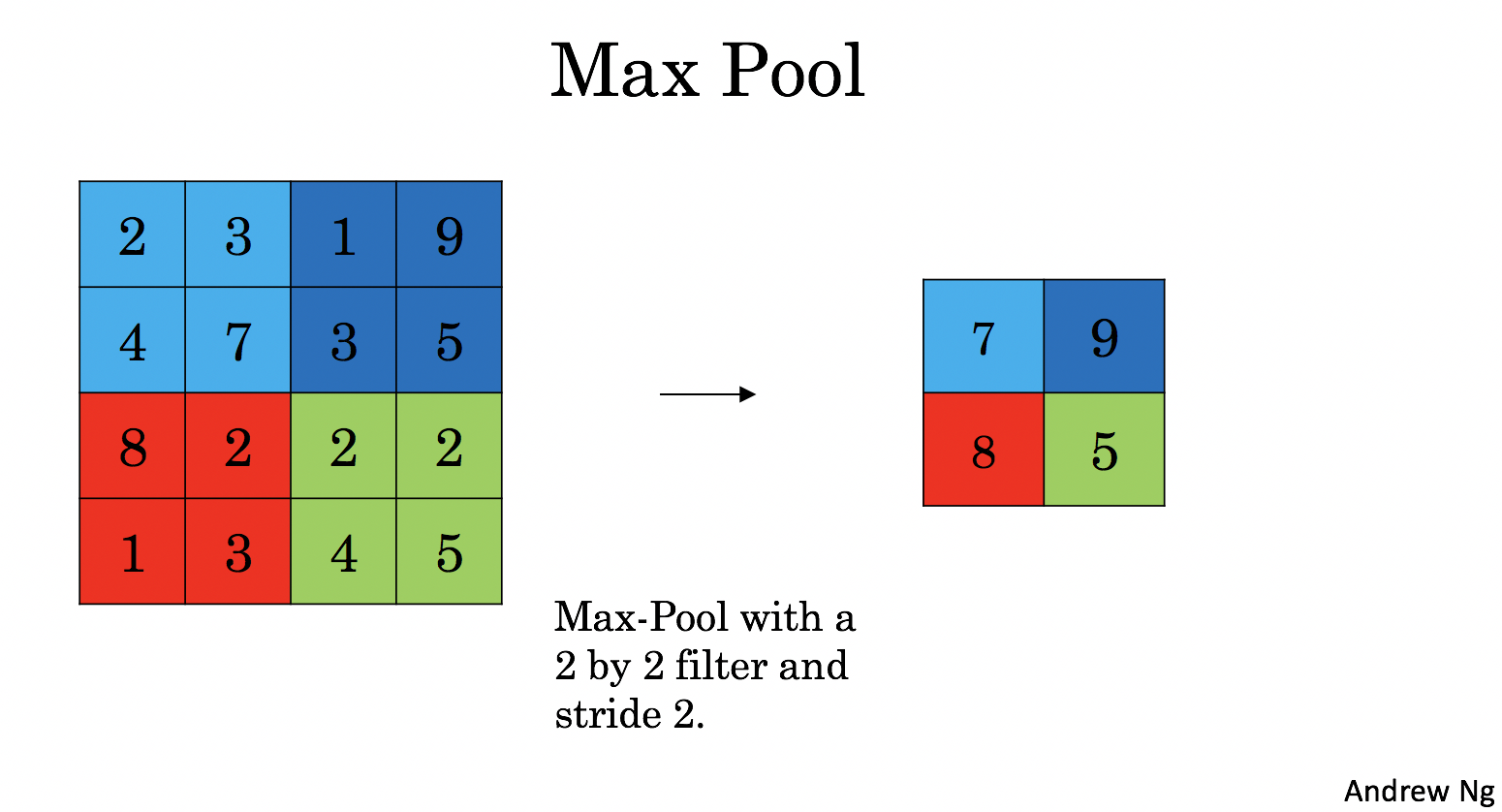
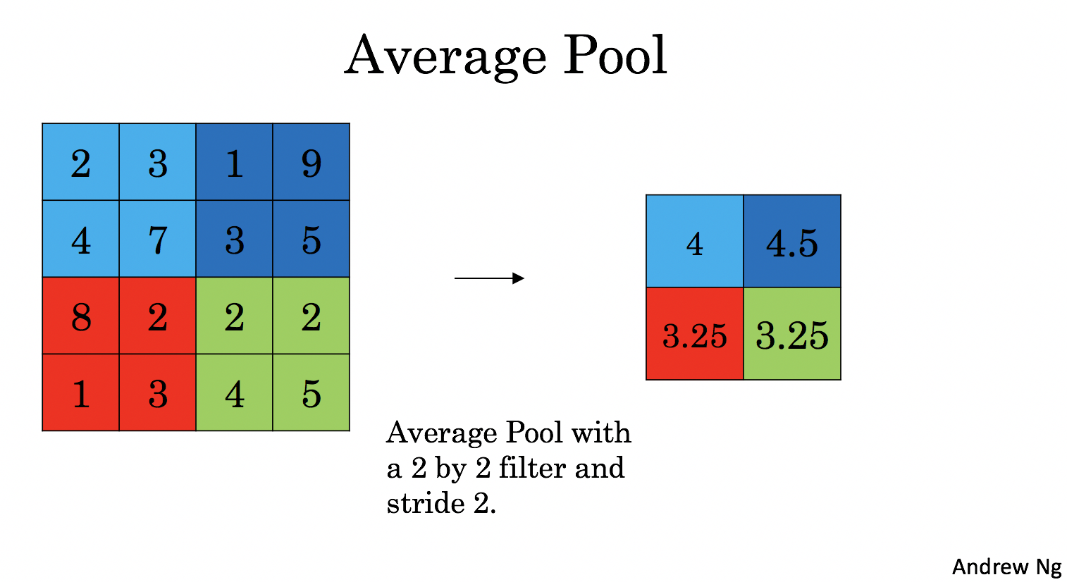
池化层(Pooling layer)减小了输入的height和width,有助于减少计算，并且有助于特征检测在输入位置的不变，两种Pooling Layers:

• Max-pooling layer: slides an (\(f, f\)) window over the input and stores the max value of the window in the output.

• Average-pooling layer: slides an (\(f, f\)) window over the input and stores the average value of the window in the output.

池化层(Pooling layers)没有反向传播训练参数，他们有 超参数：window size \(f\). 它指定计算fxf窗口max or average的 height和width.

4.1 - Forward Pooling

implement MAX-POOL and AVG-POOL, in the same function.

Exercise: Implement the forward pass of the pooling layer. Follow the hints in the comments below.

Reminder:

As there's no padding, the formulas binding the output shape of the pooling to the input shape is:

\[n_H = \lfloor \frac{n_{H_{prev}} - f}{stride} \rfloor +1
\]

\[n_W = \lfloor \frac{n_{W_{prev}} - f}{stride} \rfloor +1
\]

\[n_C = n_{C_{prev}}
\]

# GRADED FUNCTION: pool_forward

def pool_forward(A_prev, hparameters, mode = "max"):
    """
    Implements the forward pass of the pooling layer

    Arguments:
    A_prev -- Input data, numpy array of shape (m, n_H_prev, n_W_prev, n_C_prev)
    hparameters -- python dictionary containing "f" and "stride"
    mode -- the pooling mode you would like to use, defined as a string ("max" or "average")

    Returns:
    A -- output of the pool layer, a numpy array of shape (m, n_H, n_W, n_C)
    cache -- cache used in the backward pass of the pooling layer, contains the input and hparameters
    """

    # Retrieve dimensions from the input shape
    (m, n_H_prev, n_W_prev, n_C_prev) = A_prev.shape

    # Retrieve hyperparameters from "hparameters"
    f = hparameters['f']
    stride = hparameters['stride']

    # Define the dimensions of the output
    n_H = int((n_H_prev - f) / stride + 1)
    n_W = int((n_W_prev - f) / stride + 1)
    n_C = n_C_prev

    # Initialize output matrix A
    A = np.zeros((m, n_H, n_W, n_C))

    ### START CODE HERE ###
    for i in range(m):                         # loop over the training examples
        for h in range(n_H):                     # loop on the vertical axis of the output volume
            for w in range(n_W):                 # loop on the horizontal axis of the output volume
                for c in range (n_C):            # loop over the channels of the output volume

                    # Find the corners of the current "slice" (≈4 lines)
                    vert_start = h * stride
                    vert_end = vert_start + f
                    horiz_start = w * stride
                    horiz_end = horiz_start + f

                    # Use the corners to define the current slice on the ith training example of A_prev, channel c. (≈1 line)
                    a_prev_slice = A_prev[i, vert_start:vert_end, horiz_start:horiz_end, c]

                    # Compute the pooling operation on the slice. Use an if statment to differentiate the modes. Use np.max/np.mean.
                    if mode == "max":
                        A[i, h, w, c] = np.max(a_prev_slice)
                    elif mode == "average":
                        A[i, h, w, c] = np.mean(a_prev_slice)

    ### END CODE HERE ###

    # Store the input and hparameters in "cache" for pool_backward()
    cache = (A_prev, hparameters)

    # Making sure your output shape is correct
    assert(A.shape == (m, n_H, n_W, n_C))

    return A, cache

测试：

np.random.seed(1)
A_prev = np.random.randn(2, 4, 4, 3)
hparameters = {"stride" : 2, "f": 3}

A, cache = pool_forward(A_prev, hparameters)
print("mode = max")
print("A =", A)
print()
A, cache = pool_forward(A_prev, hparameters, mode = "average")
print("mode = average")
print("A =", A)

输出：

mode = max

A = [[[[1.74481176 0.86540763 1.13376944]]]

[[[1.13162939 1.51981682 2.18557541]]]]

mode = average

A = [[[[ 0.02105773 -0.20328806 -0.40389855]]]

[[[-0.22154621 0.51716526 0.48155844]]]]

5. Backpropagation in convolutional neural networks

5.1 Convolutional layer backward pass

5.11 Computing dA

\[dA += \sum _{h=0} ^{n_H} \sum_{w=0} ^{n_W} W_c \times dZ_{hw} \tag{1}
\]

• \(W_c\)是过滤器，\(dZ_{hw}\)是卷积层第h行第w列的使用点乘计算后的输出Z的梯度。

da_prev_pad[vert_start:vert_end, horiz_start:horiz_end, :] += W[:,:,:,c] * dZ[i, h, w, c]

5.1.2 Computing dW

This is the formula for computing \(dW_c\) (\(dW_c\) is the derivative of one filter) with respect to the loss:

\[dW_c += \sum _{h=0} ^{n_H} \sum_{w=0} ^ {n_W} a_{slice} \times dZ_{hw} \tag{2}
\]

\(dW_c\)是一个过滤器的梯度，aslice是\(Z_{ij}\)的激活值

dW[:,:,:,c] += a_slice * dZ[i, h, w, c]

5.1.3 - Computing db:

This is the formula for computing \(db\) with respect to the cost for a certain filter \(W_c\):

\[db = \sum_h \sum_w dZ_{hw} \tag{3}
\]

db[:,:,:,c] += dZ[i, h, w, c]

Exercise: Implement the conv_backward function below. You should sum over all the training examples, filters, heights, and widths. You should then compute the derivatives using formulas 1, 2 and 3 above.

def conv_backward(dZ, cache):
    """
    Implement the backward propagation for a convolution function

    Arguments:
    dZ -- gradient of the cost with respect to the output of the conv layer (Z), numpy array of shape (m, n_H, n_W, n_C)
    cache -- cache of values needed for the conv_backward(), output of conv_forward()

    Returns:
    dA_prev -- gradient of the cost with respect to the input of the conv layer (A_prev),
               numpy array of shape (m, n_H_prev, n_W_prev, n_C_prev)
    dW -- gradient of the cost with respect to the weights of the conv layer (W)
          numpy array of shape (f, f, n_C_prev, n_C)
    db -- gradient of the cost with respect to the biases of the conv layer (b)
          numpy array of shape (1, 1, 1, n_C)
    """

    ### START CODE HERE ###
    # Retrieve information from "cache"
    (A_prev, W, b, hparameters) = cache

    # Retrieve dimensions from A_prev's shape
    (m, n_H_prev, n_W_prev, n_C_prev) = A_prev.shape

    # Retrieve dimensions from W's shape
    (f, f, n_C_prev, n_C) = W.shape

    # Retrieve information from "hparameters"
    stride = hparameters["stride"]
    pad = hparameters["pad"]

    # Retrieve dimensions from dZ's shape
    (m, n_H, n_W, n_C) = dZ.shape

    # Initialize dA_prev, dW, db with the correct shapes
    dA_prev = np.zeros((m, n_H_prev, n_W_prev, n_C_prev))
    dW = np.zeros((f, f, n_C_prev, n_C))
    db = np.zeros((1, 1, 1, n_C))

    # Pad A_prev and dA_prev
    A_prev_pad = zero_pad(A_prev, pad)
    dA_prev_pad = zero_pad(dA_prev, pad)

    for i in range(m):                       # loop over the training examples

        # select ith training example from A_prev_pad and dA_prev_pad
        a_prev_pad = A_prev_pad[i]
        da_prev_pad = dA_prev_pad[i]

        for h in range(n_H):                   # loop over vertical axis of the output volume
            for w in range(n_W):               # loop over horizontal axis of the output volume
                for c in range(n_C):           # loop over the channels of the output volume

                    # Find the corners of the current "slice"
                    vert_start = h * stride
                    vert_end = vert_start + f
                    horiz_start = w * stride
                    horiz_end = horiz_start + f

                    # Use the corners to define the slice from a_prev_pad
                    a_slice = a_prev_pad[vert_start:vert_end, horiz_start:horiz_end, :]
#                     a_slice = A_prev_pad[i, vert_start:vert_end, horiz_start:horiz_end, :]

                    # Update gradients for the window and the filter's parameters using the code formulas given above
                    da_prev_pad[vert_start:vert_end, horiz_start:horiz_end, :] += W[:,:,:,c] * dZ[i, h, w, c]
#                     dA_prev_pad[i, vert_start:vert_end, horiz_start:horiz_end, :] += W[:,:,:,c] * dZ[i, h, w, c]
                    dW[:,:,:,c] += a_slice * dZ[i, h, w, c]
                    db[:,:,:,c] += dZ[i, h, w, c]

        # Set the ith training example's dA_prev to the unpaded da_prev_pad (Hint: use X[pad:-pad, pad:-pad, :])
        dA_prev[i, :, :, :] = da_prev_pad[pad:-pad, pad:-pad, :]
#         dA_prev[i, :, :, :] = dA_prev_pad[i, pad:-pad, pad:-pad, :]
    ### END CODE HERE ###

    # Making sure your output shape is correct
    assert(dA_prev.shape == (m, n_H_prev, n_W_prev, n_C_prev))

    return dA_prev, dW, db

测试：

np.random.seed(1)
dA, dW, db = conv_backward(Z, cache_conv)
print("dA_mean =", np.mean(dA))
print("dW_mean =", np.mean(dW))
print("db_mean =", np.mean(db))

dA_mean = 1.4524377775388075

dW_mean = 1.7269914583139097

db_mean = 7.839232564616838

5.2 Pooling layer - backward pass

5.2.1 Max pooling - backward pass

创建掩码矩阵（保存最大值位置）

\[ X = \begin{bmatrix}
1 && 3 \\
4 && 2
\end{bmatrix} \quad \rightarrow \quad M =\begin{bmatrix}
0 && 0 \\
1 && 0
\end{bmatrix}\tag{4}\]

ps: 4是最大值，则mask中相应位置为1; 其他值不是最大值，则为0

Exercise: Implement create_mask_from_window(). This function will be helpful for pooling backward.

Hints:

• np.max() may be helpful. It computes the maximum of an array.
• If you have a matrix X and a scalar x: A = (X == x) will return a matrix A of the same size as X such that:

A[i,j] = True if X[i,j] = x
A[i,j] = False if X[i,j] != x

• Here, you don't need to consider cases where there are several maxima in a matrix.

def create_mask_from_window(x):
    """
    Creates a mask from an input matrix x, to identify the max entry of x.

    Arguments:
    x -- Array of shape (f, f)

    Returns:
    mask -- Array of the same shape as window, contains a True at the position corresponding to the max entry of x.
    """

    ### START CODE HERE ### (≈1 line)
    mask = (x == np.max(x))
    ### END CODE HERE ###

    return mask

测试:

np.random.seed(1)
x = np.random.randn(2,3)
mask = create_mask_from_window(x)
print('x = ', x)
print("mask = ", mask)

x = [[ 1.62434536 -0.61175641 -0.52817175]

[-1.07296862 0.86540763 -2.3015387 ]]

mask = [[ True False False]

[False False False]]

Why do we keep track of the position of the max?

• It's because this is the input value that ultimately influenced the output, and therefore the cost.

• Backprop is computing gradients with respect to the cost, so anything that influences the ultimate cost should have a non-zero gradient.

• So, backprop will "propagate" the gradient back to this particular input value that had influenced the cost.

5.2.2 Average pooling - backward pass

均值池化层的反向传播：

\[ dZ = 1 \quad \rightarrow \quad dZ =\begin{bmatrix}
1/4 && 1/4 \\
1/4 && 1/4
\end{bmatrix}\tag{5}\]

This implies that each position in the \(dZ\) matrix contributes equally to output because in the forward pass, we took an average.

Exercise: Implement the function below to equally distribute a value dz through a matrix of dimension shape. Hint

def distribute_value(dz, shape):
    """
    Distributes the input value in the matrix of dimension shape

    Arguments:
    dz -- input scalar
    shape -- the shape (n_H, n_W) of the output matrix for which we want to distribute the value of dz

    Returns:
    a -- Array of size (n_H, n_W) for which we distributed the value of dz
    """

    ### START CODE HERE ###
    # Retrieve dimensions from shape (≈1 line)
    (n_H, n_W) = shape

    # Compute the value to distribute on the matrix (≈1 line)
    average = dz / (n_H * n_W)

    # Create a matrix where every entry is the "average" value (≈1 line)
    a = np.ones(shape) * average
    ### END CODE HERE ###

    return a

测试：

a = distribute_value(2, (2,2))
print('distributed value =', a)

distributed value = [[0.5 0.5]

[0.5 0.5]]

5.2.3 Putting it together: Pooling backward

compute backward propagation on a pooling layer.

Exercise: Implement the pool_backward function in both modes ("max" and "average").

• You will once again use 4 for-loops (iterating over training examples, height, width, and channels).

• You should use an if/elif statement to see if the mode is equal to 'max' or 'average'.

• If it is equal to 'average' you should use the distribute_value() function you implemented above to create a matrix of the same shape as a_slice.

• Otherwise, the mode is equal to 'max', and you will create a mask with create_mask_from_window() and multiply it by the corresponding value of dZ.

def pool_backward(dA, cache, mode = "max"):
    """
    Implements the backward pass of the pooling layer

    Arguments:
    dA -- gradient of cost with respect to the output of the pooling layer, same shape as A
    cache -- cache output from the forward pass of the pooling layer, contains the layer's input and hparameters
    mode -- the pooling mode you would like to use, defined as a string ("max" or "average")

    Returns:
    dA_prev -- gradient of cost with respect to the input of the pooling layer, same shape as A_prev
    """

    ### START CODE HERE ###

    # Retrieve information from cache (≈1 line)
    (A_prev, hparameters) = cache

    # Retrieve hyperparameters from "hparameters" (≈2 lines)
    stride = hparameters['stride']
    f = hparameters['f']

    # Retrieve dimensions from A_prev's shape and dA's shape (≈2 lines)
    m, n_H_prev, n_W_prev, n_C_prev = A_prev.shape
    m, n_H, n_W, n_C = dA.shape

    # Initialize dA_prev with zeros (≈1 line)
    dA_prev = np.zeros(A_prev.shape)

    for i in range(m):                       # loop over the training examples
        # select training example from A_prev (≈1 line)
        a_prev = A_prev[i]
        for h in range(n_H):                   # loop on the vertical axis
            for w in range(n_W):               # loop on the horizontal axis
                for c in range(n_C):           # loop over the channels (depth)
                    # Find the corners of the current "slice" (≈4 lines)
                    vert_start = h * stride
                    vert_end = vert_start + f
                    horiz_start = w * stride
                    horiz_end = horiz_start + f

                    # Compute the backward propagation in both modes.
                    if mode == "max":
                        # Use the corners and "c" to define the current slice from a_prev (≈1 line)
                        a_prev_slice = a_prev[vert_start:vert_end, horiz_start:horiz_end, c]
#                         a_prev_slice = A_prev[i, vert_start:vert_end, horiz_start:horiz_end, c]
                        # Create the mask from a_prev_slice (≈1 line)
                        mask = create_mask_from_window(a_prev_slice)
                        # Set dA_prev to be dA_prev + (the mask multiplied by the correct entry of dA) (≈1 line)
                        dA_prev[i, vert_start:vert_end, horiz_start:horiz_end, c] += np.multiply(mask, dA[i, h, w, c])

                    elif mode == "average":
                        # Get the value a from dA (≈1 line)
                        da = dA[i, h, w, c]
                        # Define the shape of the filter as fxf (≈1 line)
                        shape = (f, f)
                        # Distribute it to get the correct slice of dA_prev. i.e. Add the distributed value of da. (≈1 line)
                        dA_prev[i, vert_start:vert_end, horiz_start:horiz_end, c] += distribute_value(da, shape)

    ### END CODE ###

    # Making sure your output shape is correct
    assert(dA_prev.shape == A_prev.shape)

    return dA_prev

测试：

np.random.seed(1)
A_prev = np.random.randn(5, 5, 3, 2)
hparameters = {"stride" : 1, "f": 2}
A, cache = pool_forward(A_prev, hparameters)
dA = np.random.randn(5, 4, 2, 2)

dA_prev = pool_backward(dA, cache, mode = "max")
print("mode = max")
print('mean of dA = ', np.mean(dA))
print('dA_prev[1,1] = ', dA_prev[1,1])
print()
dA_prev = pool_backward(dA, cache, mode = "average")
print("mode = average")
print('mean of dA = ', np.mean(dA))
print('dA_prev[1,1] = ', dA_prev[1,1])

mode = max

mean of dA = 0.14571390272918056

dA_prev[1,1] = [[ 0. 0. ]

[ 5.05844394 -1.68282702]

[ 0. 0. ]]

mode = average

mean of dA = 0.14571390272918056

dA_prev[1,1] = [[ 0.08485462 0.2787552 ]

[ 1.26461098 -0.25749373]

[ 1.17975636 -0.53624893]]