[线性代数] 线性代数入门A Gentle Introduction

An Overview: System of Linear Equations

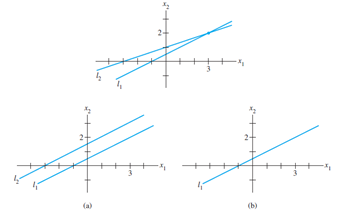
Basically, linear algebra solves system of linear equations (where variables/unknowns are linear with power of 1). Our aim is to find a vector solution which satisfy a system of linear equations, which is a collection of many linear equations. Some system is consistent (having one or more solution vector(s)), while some are not. When we treat each equation in the system as a line in some space, a consistent system allows these lines to cross in at least one point in space, and that's the solution to all linear equations within the system. What if these lines all collapse into 1 line? If so, we would have infinitely many solutions to the system as each point in intersection contribute to one possible solution in the pool and these solutions are aggregated into a solution set. The existence of AT LEAST 1 free variable in a system classify systems with a unique solution from those with infinitely many solutions.

In an inconsistent system, however, there are no solution, meaning all lines in the system do not intersect, meaning all lines do not intersect at least one point. (While some of them do intersect with some another, but no lines intersect with all lines).

Solving and Evaluating the System

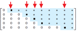
With all these terminologies in mind, how could we start finding the solution set for a complicated system involving lots of linear equations? A system is solved by matrix transformation, where we transform more complicated system into row equivalent ones via elementary row operations on AUGMENTED matrices, turning them into reduced row echelon forms. The red arrow shows the pivot columns in the general echelon form of a matrix. Each pivot is used to generates zeros within the same columns (be it above/below the pivot entry, as rows are interchangeable guaranteed by the algorithm). However, sometimes the row operations to generate reduced row echelon forms could become a bit too involved when we only need to get a grip of the nature of solution set (i.e. is there any solutions to the system? If so, is solution unique?).

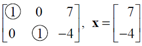
The following is an example of row-reducing an augmented matrix and it yields 2 pivot columns, each corresponds to one of the variables in the system. Thus, there exists no free variables and we get the unique solution to the system as

Linear Combination

Linear combination combines vectors together with coefficient, and to generate a new vector. The a_i below refers to columns in any, same dimension and x_i simply acts as coefficients to linearly transform the columns they adhere to. A span of a set of vectors means the space generated by ALL possible linear combinations of those vectors. If b equals to left hand side, it is within the space spanned by a_i.

The equations above can also be expressed as matrix equation below. Ax has a solution iff b is a linear combination of columns in A. If A has a pivot position at each row, its columns span the space, where any vector b within satisfy Ax=b.

Homogeneity of System

A system can be classified into homogeneous or nonhomogeneous based on different results from matrix equation. Ax=0 belongs to homogeneous system and Ax=b belongs to nonhomogeneous system. After all these definitions, our goal is to identify the solution set.

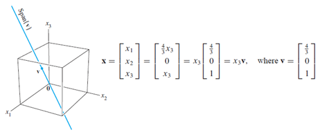
Solution to Ax=0 can either be trivial or non-trivial if there exist at least one free variable. Suppose we solve a homogeneous system and yield solution x as the following. There exists one free variable x₃, literally allowing the solution to span a space of R³. Noted here the solution x has been expressed in parametric vector form.

Non-homogeneous System

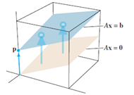
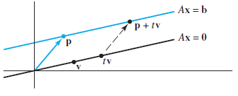
Non-homogeneous system refers to system is expressed as Ax=b, where b!=0. This hints it must contain non-trivial solution. Indeed, the solution set of such system can be expressed as a linear combination of a vector, plus the solution set for the corresponding homogeneous solution, as illustrated below. V is ANY solution to the homogeneous system, while p is one of the system for where Ax=b is consistent. Thus, any pair of combination of (x,v_h) forms a nontrivial solution to the nonhomogeneous system.

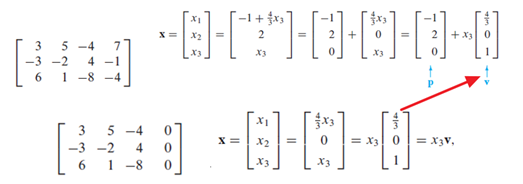
Geometrically, solutions to homogeneous system is just a subset of that for nonhomogeneous ones.

Linear independence

only exists trivial solution. From the expression we know that to verify linear independence, we rely on row-reducing homogeneous system. In case of non-trivial solution, there must exists MORE THAN AT LEAST ONE non-zero weights in the expression. A set of vectors is linearly dependent when some of vectors in the set are within the span of others. A set containing v=0 must be linearly dependent, as its weight can be any non-zero numbers but still gives cv=0.

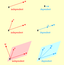
From the definition of linear independence, identifying such dependence on a set of vectors is equivalent to solving a homogeneous system. Each non-trivial solution contributes to one linear dependence among equations within the system. Meanwhile, when there are only basic variables and no free variables in the system, Ax=0 has only trivial solution, column vectors in A are therefore linearly independent.

When the idea of linear independence is extended to set, a set is defined as linearly dependent set if AT LEAST ONE vector in the set is the linear combination of others. In other words, some vector in the set may still fail to be the linear combination of others, but the set can still be linearly dependent.

Another quick test on a set without resorting to solving homogeneous system is of the following. For a set whose elements have a dimension of n, the set becomes linearly dependent if p>n. The proof is trivial.

Indeed, the concept of linear independence in two vectors could be easily generalized into an ordered set with many vectors. The following shows two vectors are linearly dependent when one vector is a scalar multiple of another, meaning the coefficient for one of the vectors is non-zero, which corresponds to a non-trivial solution to Ax=0 when these vectors are packed to form columns of A. Given the following v₁ (6,2) and v₂ (3,1) are linearly dependent, there exists a pair of coefficients where v₁ and v₂ cancels out each other. For example, when -2v₂ we get v₃=(-6,-2), rendering v₁+v₃=0=(1)v₁+(-2)v₂! This gives us some intuition about why testing linear independence involves solving for homogenous systems! BECAUSE DEPENDENT VECTORS GET CANCELLED OUT!!!

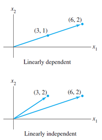
The same notion can be expanded into a set of multiple vectors as well, but in a relaxed manner. An ordered set of vectors must be linearly dependent if there's AT LEAST ONE vector in the set expressible as a linear combination of (some/all of the) other vectors. However, when the notion above is being generalized in a set with multiple vectors, it is not required for a vector to be the linear combination of ALL OTHER vectors within the set. Thus, this is a more relaxed formulation of linear dependence.

Linear Transformation

What is linear transformation exactly? A transformation is linear if the following is observed.

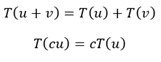
If a given transformation is linear, then the following is true:

Superposition principle:

So far, we view matrix equation as a linear combination of columns with coefficient/solution x. Indeed, there is another interpretation of matrix equation: linear transformation. For instance, gives two interpretations as following.

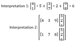
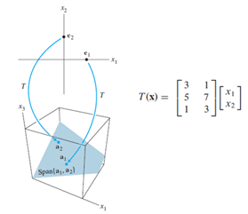
This new idea allows us to transform/maps any vector from domain with Rⁿ to a codomain R^m. Effectively, by controlling the dimension of the standard matrix, we could transform a vector into the same dimensional space. Thus, any vectors (image) in the range is a linear combination of the standard matrix and therefore, the range is spanned by Ax, with all possible x defined in the domain. The transformation does not necessarily expands the dimensional space of a vector, but instead shrinks it, as illustrated by this interesting example, which maps a vector in R³ onto a plane.

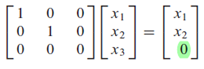
One application of linear transformation is to identify if a vector is an image/fall within the range of a linear transformation. This is equivalent to solving nonhomogeneous system, i.e. when the system is consistent, the vector is an image to the transformation.

The standard matrix

The standard matrix can be uniquely identified by a matrix A in a form of . This notion links transformation and matrix equation together. But how could we find such a standard matrix? First, recall the superposition property of a linear transformation T and note that a vector could be expressed as an identity matrix, e, of itself:

When applied a transformation, we get

So we could conclude the following, where the standard matrix is unique determined by applying transformations on columns in identity matrix

and the transformation on x becomes a matrix equation

T(x) = Ax

Therefore, the standard matrix is recoverable iff T(e_i) is given.

Mapping: Onto and one-to-one

Onto and one-to-one describe the relation of mapping between b in R^m and x from the domain. Onto requires b to be an image of at least one x in domain Rⁿ, this effectively eliminates those b whose falls out of the range of the transformation. However, this restriction is relaxed in 'one-to-one', where b could be mapped to at most one of x in Rⁿ, this includes those b who is in codomain, but not within range of the transformation.

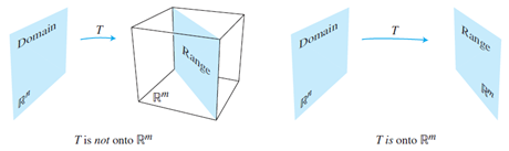
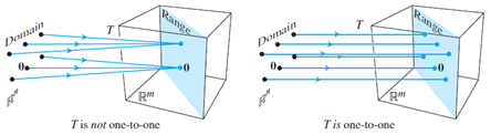
But how could we tell from a given standard matrix whether it provides a one-to-one or onto mapping? Well, that's easy. We just need to apply row transformations to get the reduced echelon form, identify the basic and free variables. For example, given the following standard matrix:

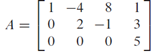
It is apparently in echelon form with one single free variable, meaning as input could be of any scalar, thus we have multiple inputs which give the same result T(x), meaning b can be a result of multiple x inputs. This suggests the transformation itself is not a one-to-one mapping. Noted here it does not necessarily mean this transformation gives onto mapping, as we are not sure if the transformation's codomain equal to its range or not. We can also draw a conclusion as follow. The transformation is:

1. one-to-one if Ax=0 has only trivial solution.
2. Onto if a_i span R^m à i.e. codomain same as range
3. One-to-one if a_i linearly independent à all are basic variables; the system is consistent with only unique solution.

Let's look at the following transformation. The columns are apparently linearly independent as none of them is a multiple of each other, so this transformation is one-to-one. However, since m<n, the columns of A do not span R³, thus, the mapping from R² to R³ is not onto, as

Some Examples

Ex#1 The following shows an augmented matrix. Despite it is a system of 3 linear equations with 2 unknowns, v=[0,4,4] still spans the coefficient matrix, as the system is consistent, meaning v is a linear combination of columns in A. The last row in the echelon form means after row operations, the 3^rd equation is eliminated from the system, thus, it should not affect the span, where we only consider a system is consistent or not.

Ex#2 For a coefficient matrix as below, since not every row has a pivot position, (in this case, there's a zero row) meaning that for non-zero entry in b corresponding to the zero row in A, the system would become inconsistent. Therefore, that b cannot be expressed as a linear combination of a_i, and Thus, all the a_i do not span R^m, which is R⁴ (not R³!) in this case. This also means that for some b, Ax=b is inconsistent. Noted here we only consider COEFFICIENT matrix, NOT AUGMENTED ONES. Augmented ones are used iff we are to identify solutions from the system.

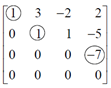
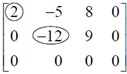
Ex#3 Not every column in the augmented matrix below is a pivot column. Thus, there exists free variable, which is x₃ in this case, granting the entire homogeneous system non-trivial solutions.

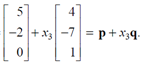
Ex#4 The following represent a line passing via point p in the direction of q.

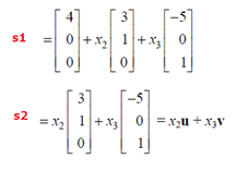
Ex#5 Both s1 and s2 represents a plane in R³. But s1 is a plane which is parallel to s2 and pass through the point v=[4,0,0]. Apparently, s1 is the solution for Ax=b and s2 is for Ax=0. Noted the dimension in any vector down there has ZERO correlation with the geometry of the solution, but it just specifies the space R^m. For instance, all the vectors in following exist in R³ but the vectors just span a 2-d plane in a 3-d space (as there are just two free variables).

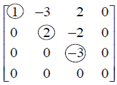
Ex#6 Despite each a_i in the following augmented matrix is in R⁴, each of these columns are pivot columns, and the homogeneous system only has trivial solution. Thus, the a_i are linearly independent.

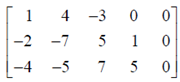
Ex#7 You may not want to row-reduce the following to decide if the columns are linearly independence. Since each column is in R³ and we have only 3 rows, there are at most 3 pivot positions only. However, there exists 4 columns. This means one of the variables must be free variable and Ax=0 has nontrivial solution. The columns in the set is thus linearly dependent.

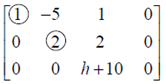
Ex#8 The following has nontrivial solution when h=-10 as x₃ is free. Thus, the columns are linearly dependent when h+10=0.

Ex#9 This linear transformation maps a vector to a point as T(p) if v=0; otherwise, it produces a line passing via T(p) with direction as T(v).

Ex#10 If a linear transformation is applied on x=su+tv, yields T(x)=sT(u)+tT(v). The set of images span {T(u), T(v)}. There are 3 possible cases for interpreting the span.

1. If T(u), T(v) linearly independent, span=a plane passing T(u), T(v) and 0.
2. If T(u), T(v) not both zero and linearly dependent, span=a line passing through 0
3. If T(u)=T(v)=0, span={0}

Ex#11 If {v₁,v₂,v₃} are linearly independent and given a linear transformation T, then {T(v₁), T(v₂), T(v₃)} are also linearly independent. Since:

c₁v₁+c₂v₂+c₃v₃=0, not all c_i=0

Similarly, due to linearity of transformation,

T(c₁v₁)+T(c₂v₂)+T(c₃v₃) = c₁T(v₁)+c₂T(v₂)+c₃T(v₃) = 0, not all c_i=0

Thus, the set {T(v₁), T(v₂), T(v₃)} is also linearly independent.

Ex#12 Given a linear transformation Find x so that T(x₁,x₂)=(3,8). Fortunately, the system gives unique solution, indicating a one-to-one mapping of x to T(x). Otherwise, if a system contains free variables, there would be several solutions giving T(x) = (3,8).

Ex#13 For a linear transformation from R³àR⁴ cannot be onto, as columns in the corresponding standard 3x4 matrix does not span across R⁴. Here we only have 3 pivot columns possible and which, apparently, do not span R⁴. However, we cannot immediately conclude this function is one-to-one, unless we also prove these columns are linearly independent as well.

Recall for a function to be 'onto', its range must equal to its codomain. Suppose codomain is of R^m, we must at least have m linearly independent columns for this function to be onto, as this is when the columns span R^m.