朴素贝叶斯(Naive Bayesian)

• 简介

Naive Bayesian算法 也叫朴素贝叶斯算法（或者称为傻瓜式贝叶斯分类）

朴素（傻瓜）：特征条件独立假设

贝叶斯：基于贝叶斯定理

这个算法确实十分朴素（傻瓜），属于监督学习,它是一个常用于寻找决策面的算法。

• 基本思想

（1）病人分类举例

有六个病人 他们的情况如下：

症状	职业	病名
打喷嚏	护士	感冒
打喷嚏	农夫	过敏
头痛	建筑工人	脑震荡
头痛	建筑工人	感冒
打喷嚏	教师	感冒
头痛	教师	脑震荡

根据这张表 如果来了第七个病人 他是一个 打喷嚏 的 建筑工人

那么他患上感冒的概率是多少

根据贝叶斯定理：

P(A|B) = P(B|A) P(A) / P(B)

可以得到：

P(感冒|打喷嚏x建筑工人) = P(打喷嚏x建筑工人|感冒) x P(感冒) / P(打喷嚏x建筑工人)

假定 感冒 与 打喷嚏 相互独立 那么上面的等式变为：

P(感冒|打喷嚏x建筑工人) = P(打喷嚏|感冒) x P(建筑工人|感冒) x P(感冒) / （ P(打喷嚏) x P(建筑工人) ）
P(感冒|打喷嚏x建筑工人) = 2/3 x 1/3 x 1/2 /（ 1/2 x 1/3 ）= 2/3

因此 这位打喷嚏的建筑工人 患上感冒的概率大约是66%

（2）朴素贝叶斯分类器公式

假设某个体有n项特征，分别为F1、F2、…、Fn。现有m个类别，分别为C1、C2、…、Cm。贝叶斯分类器就是计算出概率最大的那个分类，也就是求下面这个算式的最大值：

P(C|F1 x F2 ...Fn) = P(F1 x F2 ... Fn|C) x P(C) / P(F1 x F2 ... Fn)

由于 P(F1xF2 … Fn) 对于所有的类别都是相同的，可以省略，问题就变成了求

P(F1 x F2 ... Fn|C)P(C)

的最大值

根据朴素贝叶斯的朴素特点（特征条件独立假设），因此：

P(F1 x F2 ... Fn|C)P(C) = P(F1|C) x P(F2|C) ... P(Fn|C)P(C)

上式等号右边的每一项，都可以从统计资料中得到，由此就可以计算出每个类别对应的概率，从而找出最大概率的那个类。

• 代码实现

环境：MacOS mojave　　10.14.3

Python　　3.7.0

使用库：scikit-learn    0.19.2

在终端输入下面的代码安装sklearn

pip install sklearn

sklearn库官方文档http://scikit-learn.org/stable/modules/generated/sklearn.naive_bayes.GaussianNB.html

>>> import numpy as np
>>> X = np.array([[-1, -1], [-2, -1], [-3, -2], [1, 1], [2, 1], [3, 2]])
>>> Y = np.array([1, 1, 1, 2, 2, 2])
#生成六个训练点，其中前三个属于标签（分类）1 后三个属于标签（分类）2
>>> from sklearn.naive_bayes import GaussianNB
#导入外部模块
>>> clf = GaussianNB()#创建高斯分类器，把GaussianNB赋值给clf（分类器）
>>> clf.fit(X, Y)#开始训练
#它会学习各种模式，然后就形成了我们刚刚创建的分类器（clf）
#我们在分类器上调用fit函数，接下来将两个参数传递给fit函数，一个是特征x 一个是标签y#最后我们让已经完成了训练的分类器进行一些预测，我们为它提供一个新点[-0.8,-1]
>>> print(clf.predict([[-0.8, -1]]))
[1]

上面的流程为：创建训练点->创建分类器->进行训练->对新的数据进行分类

上面的新的数据属于标签（分类）2

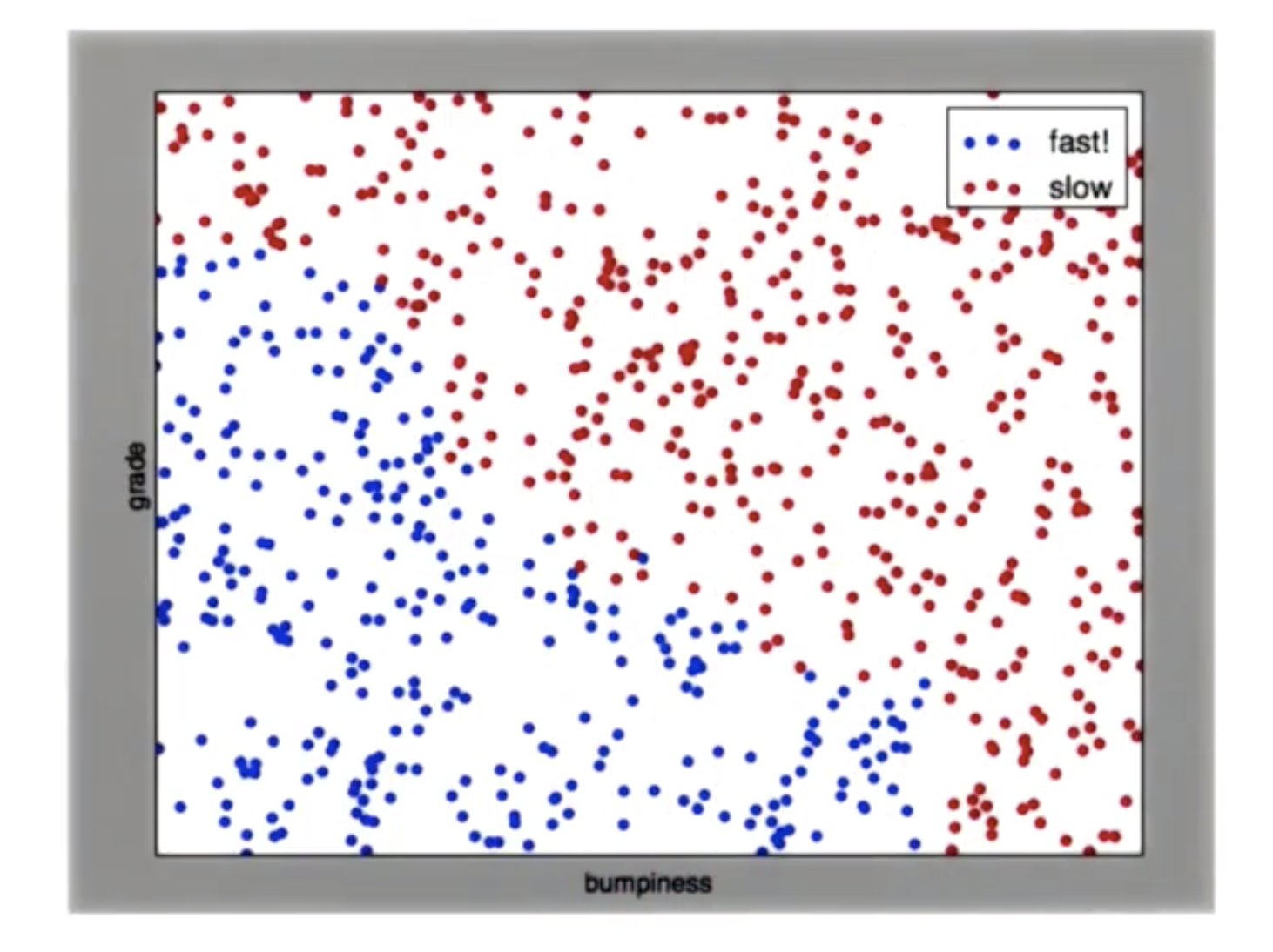
• 绘制决策面

对于给定的一副散点图，其中蓝色是慢速区 红色是快速区，如何画出一条线 将点分开

perp_terrain_data.py

生成训练点

import random

def makeTerrainData(n_points=1000):
###############################################################################
### make the toy dataset
    random.seed(42)
    grade = [random.random() for ii in range(0,n_points)]
    bumpy = [random.random() for ii in range(0,n_points)]
    error = [random.random() for ii in range(0,n_points)]
    y = [round(grade[ii]*bumpy[ii]+0.3+0.1*error[ii]) for ii in range(0,n_points)]
    for ii in range(0, len(y)):
        if grade[ii]>0.8 or bumpy[ii]>0.8:
            y[ii] = 1.0

### split into train/test sets
    X = [[gg, ss] for gg, ss in zip(grade, bumpy)]
    split = int(0.75*n_points)
    X_train = X[0:split]
    X_test  = X[split:]
    y_train = y[0:split]
    y_test  = y[split:]

    grade_sig = [X_train[ii][0] for ii in range(0, len(X_train)) if y_train[ii]==0]
    bumpy_sig = [X_train[ii][1] for ii in range(0, len(X_train)) if y_train[ii]==0]
    grade_bkg = [X_train[ii][0] for ii in range(0, len(X_train)) if y_train[ii]==1]
    bumpy_bkg = [X_train[ii][1] for ii in range(0, len(X_train)) if y_train[ii]==1]

#    training_data = {"fast":{"grade":grade_sig, "bumpiness":bumpy_sig}
#            , "slow":{"grade":grade_bkg, "bumpiness":bumpy_bkg}}

    grade_sig = [X_test[ii][0] for ii in range(0, len(X_test)) if y_test[ii]==0]
    bumpy_sig = [X_test[ii][1] for ii in range(0, len(X_test)) if y_test[ii]==0]
    grade_bkg = [X_test[ii][0] for ii in range(0, len(X_test)) if y_test[ii]==1]
    bumpy_bkg = [X_test[ii][1] for ii in range(0, len(X_test)) if y_test[ii]==1]

    test_data = {"fast":{"grade":grade_sig, "bumpiness":bumpy_sig}
            , "slow":{"grade":grade_bkg, "bumpiness":bumpy_bkg}}

    return X_train, y_train, X_test, y_test
#    return training_data, test_data

ClassifyNB.py

高斯分类

def classify(features_train, labels_train):
    ### import the sklearn module for GaussianNB
    ### create classifier
    ### fit the classifier on the training features and labels
    ### return the fit classifier

    from sklearn.naive_bayes import GaussianNB
    clf = GaussianNB()
    clf.fit(features_train, labels_train)
    return clf
    pred = clf.predict(features_test)
    

class_vis.py

绘图与保存图像

import warnings
warnings.filterwarnings("ignore")

import matplotlib
matplotlib.use('agg')

import matplotlib.pyplot as plt
import pylab as pl
import numpy as np

#import numpy as np
#import matplotlib.pyplot as plt
#plt.ioff()

def prettyPicture(clf, X_test, y_test):
    x_min = 0.0; x_max = 1.0
    y_min = 0.0; y_max = 1.0

    # Plot the decision boundary. For that, we will assign a color to each
    # point in the mesh [x_min, m_max]x[y_min, y_max].
    h = .01  # step size in the mesh
    xx, yy = np.meshgrid(np.arange(x_min, x_max, h), np.arange(y_min, y_max, h))
    Z = clf.predict(np.c_[xx.ravel(), yy.ravel()])

    # Put the result into a color plot
    Z = Z.reshape(xx.shape)
    plt.xlim(xx.min(), xx.max())
    plt.ylim(yy.min(), yy.max())

    plt.pcolormesh(xx, yy, Z, cmap=pl.cm.seismic)

    # Plot also the test points
    grade_sig = [X_test[ii][0] for ii in range(0, len(X_test)) if y_test[ii]==0]
    bumpy_sig = [X_test[ii][1] for ii in range(0, len(X_test)) if y_test[ii]==0]
    grade_bkg = [X_test[ii][0] for ii in range(0, len(X_test)) if y_test[ii]==1]
    bumpy_bkg = [X_test[ii][1] for ii in range(0, len(X_test)) if y_test[ii]==1]

    plt.scatter(grade_sig, bumpy_sig, color = "b", label="fast")
    plt.scatter(grade_bkg, bumpy_bkg, color = "r", label="slow")
    plt.legend()
    plt.xlabel("bumpiness")
    plt.ylabel("grade")

    plt.savefig("test.png")

Main.py

主程序

from prep_terrain_data import makeTerrainData
from class_vis import prettyPicture
from ClassifyNB import classify

import numpy as np
import pylab as pl

features_train, labels_train, features_test, labels_test = makeTerrainData()

### the training data (features_train, labels_train) have both "fast" and "slow" points mixed
### in together--separate them so we can give them different colors in the scatterplot,
### and visually identify them
grade_fast = [features_train[ii][0] for ii in range(0, len(features_train)) if labels_train[ii]==0]
bumpy_fast = [features_train[ii][1] for ii in range(0, len(features_train)) if labels_train[ii]==0]
grade_slow = [features_train[ii][0] for ii in range(0, len(features_train)) if labels_train[ii]==1]
bumpy_slow = [features_train[ii][1] for ii in range(0, len(features_train)) if labels_train[ii]==1]

clf = classify(features_train, labels_train)

### draw the decision boundary with the text points overlaid
prettyPicture(clf, features_test, labels_test)

运行得到分类完成图像：

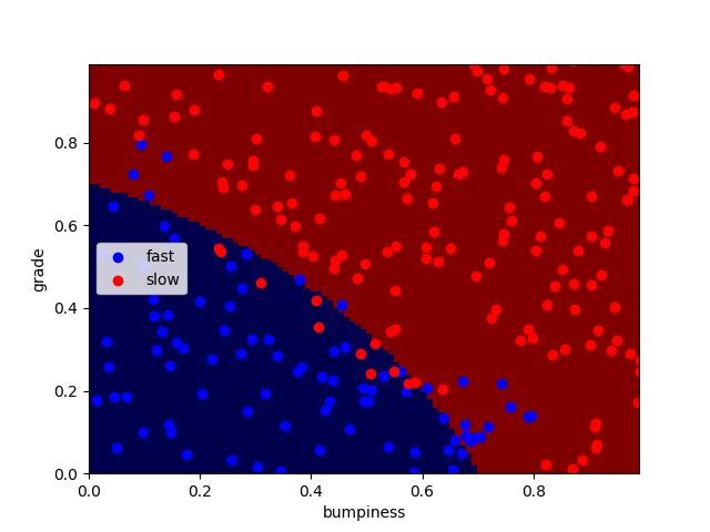
可以看到并不是所有的点都正确分类了，还有一小部分点被错误分类了

计算分类正确率：

accuracy.py

from class_vis import prettyPicture
from prep_terrain_data import makeTerrainData
from classify import NBAccuracy

import matplotlib.pyplot as plt
import numpy as np
import pylab as pl

features_train, labels_train, features_test, labels_test = makeTerrainData()

def submitAccuracy():
    accuracy = NBAccuracy(features_train, labels_train, features_test, labels_test)
    return accuracy

在主程序Main结尾加入一段：

from studentCode import submitAccuracy
print(submitAccuracy())

得到正确率：0.884

• 朴素贝叶斯的优势与劣势

优点：1、非常易于执行　　2、它的特征空间非常大　　3、运行非常容易、非常有效

缺点：它会与间断、由多个单词组成且意义明显不同的词语不太适合（eg：芝加哥公牛）