Tutorial: Implementation of Siamese Network on Caffe, Torch, Tensorflow

Tutorial: Implementation of Siamese Network with Caffe, Theano, PyTorch, Tensorflow 

Updated on 2018-07-23 14:33:23

---

　　1. caffe version: 

　　　　If you want to try this network, just do as the offical document said, like the following codes:  　　

 ---
 title: Siamese Network Tutorial
 description: Train and test a siamese network on MNIST data.
 category: example
 include_in_docs: true
 layout: default
 priority:
 ---

 # Siamese Network Training with Caffe
 This example shows how you can use weight sharing and a contrastive loss
 function to learn a model using a siamese network in Caffe.

 We will assume that you have caffe successfully compiled. If not, please refer
 to the [Installation page](../../installation.html). This example builds on the
 [MNIST tutorial](mnist.html) so it would be a good idea to read that before
 continuing.

 *The guide specifies all paths and assumes all commands are executed from the
 root caffe directory*

 ## Prepare Datasets

 You will first need to download and convert the data from the MNIST
 website. To do this, simply run the following commands:

     ./data/mnist/get_mnist.sh
     ./examples/siamese/create_mnist_siamese.sh

 After running the script there should be two datasets,
 `./examples/siamese/mnist_siamese_train_leveldb`, and
 `./examples/siamese/mnist_siamese_test_leveldb`.

 ## The Model
 First, we will define the model that we want to train using the siamese network.
 We will use the convolutional net defined in
 `./examples/siamese/mnist_siamese.prototxt`. This model is almost
 exactly the same as the [LeNet model](mnist.html), the only difference is that
 we have replaced the top layers that produced probabilities over the  digit
 classes with a linear "feature" layer that produces a  dimensional vector.

     layer {
       name: "feat"
       type: "InnerProduct"
       bottom: "ip2"
       top: "feat"
       param {
         name: "feat_w"
         lr_mult:
       }
       param {
         name: "feat_b"
         lr_mult:
       }
       inner_product_param {
         num_output:
       }
     }

 ## Define the Siamese Network

 In this section we will define the siamese network used for training. The
 resulting network is defined in
 `./examples/siamese/mnist_siamese_train_test.prototxt`.

 ### Reading in the Pair Data

 We start with a data layer that reads from the LevelDB database we created
 earlier. Each entry in this database contains the image data for a pair of
 images (`pair_data`) and a binary label saying if they belong to the same class
 or different classes (`sim`).

     layer {
       name: "pair_data"
       type: "Data"
       top: "pair_data"
       top: "sim"
       include { phase: TRAIN }
       transform_param {
         scale: 0.00390625
       }
       data_param {
         source: "examples/siamese/mnist_siamese_train_leveldb"
         batch_size:
       }
     }

 In order to pack a pair of images into the same blob in the database we pack one
 image per channel. We want to be able to work with these two images separately,
 so we add a slice layer after the data layer. This takes the `pair_data` and
 slices it along the channel dimension so that we have a single image in `data`
 and its paired image in `data_p.`

     layer {
       name: "slice_pair"
       type: "Slice"
       bottom: "pair_data"
       top: "data"
       top: "data_p"
       slice_param {
         slice_dim:
         slice_point:
       }
     }

 ### Building the First Side of the Siamese Net

 Now we can specify the first side of the siamese net. This side operates on
 `data` and produces `feat`. Starting from the net in
 `./examples/siamese/mnist_siamese.prototxt` we add default weight fillers. Then
 we name the parameters of the convolutional and inner product layers. Naming the
 parameters allows Caffe to share the parameters between layers on both sides of
 the siamese net. In the definition this looks like:

     ...
     param { name: "conv1_w" ...  }
     param { name: "conv1_b" ...  }
     ...
     param { name: "conv2_w" ...  }
     param { name: "conv2_b" ...  }
     ...
     param { name: "ip1_w" ...  }
     param { name: "ip1_b" ...  }
     ...
     param { name: "ip2_w" ...  }
     param { name: "ip2_b" ...  }
     ...

 ### Building the Second Side of the Siamese Net

 Now we need to create the second path that operates on `data_p` and produces
 `feat_p`. This path is exactly the same as the first. So we can just copy and
 paste it. Then we change the name of each layer, input, and output by appending
 `_p` to differentiate the "paired" layers from the originals.

 ### Adding the Contrastive Loss Function

 To train the network we will optimize a contrastive loss function proposed in:
 Raia Hadsell, Sumit Chopra, and Yann LeCun "Dimensionality Reduction by Learning
 an Invariant Mapping". This loss function encourages matching pairs to be close
 together in feature space while pushing non-matching pairs apart. This cost
 function is implemented with the `CONTRASTIVE_LOSS` layer:

     layer {
         name: "loss"
         type: "ContrastiveLoss"
         contrastive_loss_param {
             margin: 1.0
         }
         bottom: "feat"
         bottom: "feat_p"
         bottom: "sim"
         top: "loss"
     }

 ## Define the Solver

 Nothing special needs to be done to the solver besides pointing it at the
 correct model file. The solver is defined in
 `./examples/siamese/mnist_siamese_solver.prototxt`.

 ## Training and Testing the Model

 Training the model is simple after you have written the network definition
 protobuf and solver protobuf files. Simply run
 `./examples/siamese/train_mnist_siamese.sh`:

     ./examples/siamese/train_mnist_siamese.sh

 # Plotting the results

 First, we can draw the model and siamese networks by running the following
 commands that draw the DAGs defined in the .prototxt files:

     ./python/draw_net.py \
         ./examples/siamese/mnist_siamese.prototxt \
         ./examples/siamese/mnist_siamese.png

     ./python/draw_net.py \
         ./examples/siamese/mnist_siamese_train_test.prototxt \
         ./examples/siamese/mnist_siamese_train_test.png

 Second, we can load the learned model and plot the features using the iPython
 notebook:

     ipython notebook ./examples/siamese/mnist_siamese.ipynb

　

If you want to shown the neural network in a image. first, you should install the following softwares:

　　　　1. sudo apt-get install graphviz

　　　　2. sudo pip install pydot2

then, you can draw the following graph using tool provided by python files.

　　

---

　　  If you want to know how to implement this on your own data. You should:

　　　　1. Preparing your data:

　　　　　　==>> positive and negative image pairs and corresponding label (1 and -1).

　　　　2. Convert the files into lmdb files

　　　　3. then just do as above mentioned.

　　==>>  But  I am still feel confused about how to deal with this whole process.

　　　　　　Will fill with this part later.

2. Siamese Lasagne Theano version :   

 # Run on GPU: THEANO_FLAGS=mode=FAST_RUN,device=gpu,floatX=float32 python mnist_siamese_graph.py
 from __future__ import print_function

 import sys
 import os
 import time
 import numpy as np
 import theano
 import theano.tensor as T
 import lasagne
 import utils
 from progressbar import AnimatedMarker, Bar, BouncingBar, Counter, ETA, \
     FileTransferSpeed, FormatLabel, Percentage, \
     ProgressBar, ReverseBar, RotatingMarker, \
     SimpleProgress, Timer
 import matplotlib.pyplot as plt
 from matplotlib import gridspec
 import cPickle as pickle
 import time
 from sklearn import metrics
 from scipy import interpolate
 from lasagne.regularization import regularize_layer_params_weighted, l2, l1
 from lasagne.regularization import regularize_layer_params

 NUM_EPOCHS = 40
 BATCH_SIZE = 100
 LEARNING_RATE = 0.001
 MOMENTUM = 0.9

 # def build_cnn(input_var=None):
 #     net = lasagne.layers.InputLayer(shape=(None, 1, 64, 64),
 #                                         input_var=input_var)
 #     cnn1 = lasagne.layers.Conv2DLayer(
 #             net, num_filters=96, filter_size=(7, 7),
 #             nonlinearity=lasagne.nonlinearities.rectify,
 #             W=lasagne.init.GlorotNormal())
 #     pool1 = lasagne.layers.MaxPool2DLayer(cnn1, pool_size=(2, 2))
 #     cnn2 = lasagne.layers.Conv2DLayer(
 #             pool1, num_filters=64, filter_size=(6, 6),
 #             nonlinearity=lasagne.nonlinearities.rectify,
 #             W=lasagne.init.GlorotNormal())
 #     fc1 = lasagne.layers.DenseLayer(cnn2, num_units=128)
 #     # network = lasagne.layers.FlattenLayer(fc1)
 #     return fc1

 def build_cnn(input_var=None):
     net = lasagne.layers.InputLayer(shape=(None, 1, 64, 64),
                                         input_var=input_var)
     cnn1 = lasagne.layers.Conv2DLayer(
             net, num_filters=96, filter_size=(7, 7),
             nonlinearity=lasagne.nonlinearities.rectify,
             stride = (3,3),
             W=lasagne.init.GlorotNormal())
     pool1 = lasagne.layers.MaxPool2DLayer(cnn1, pool_size=(2, 2))
     cnn2 = lasagne.layers.Conv2DLayer(
             pool1, num_filters=192, filter_size=(5, 5),
             nonlinearity=lasagne.nonlinearities.rectify,
             W=lasagne.init.GlorotNormal())
     pool2 = lasagne.layers.MaxPool2DLayer(cnn2, pool_size=(2, 2))
     cnn3 = lasagne.layers.Conv2DLayer(
             pool2, num_filters=256, filter_size=(3, 3),
             nonlinearity=lasagne.nonlinearities.rectify,
             W=lasagne.init.GlorotNormal())
     # fc1 = lasagne.layers.DenseLayer(cnn2, num_units=128)
     network = lasagne.layers.FlattenLayer(cnn3)
     return network

 def init_data(train,test):
     dtrain = utils.load_brown_dataset("/home/vassilis/Datasets/"+train+"/")
     dtest = utils.load_brown_dataset("/home/vassilis/Datasets/"+test+"/")

     dtrain['patches'] = dtrain['patches'].astype('float32')
     dtest['patches'] = dtest['patches'].astype('float32')

     dtrain['patches'] /= 255
     dtest['patches'] /= 255

     mu = dtrain['patches'].mean()
     dtrain['patches'] = dtrain['patches'] - mu
     dtest['patches'] = dtest['patches'] - mu
     return dtrain,dtest

 def eval_test(net,d):
     bs = 100
     pb = np.array_split(d['patches'],bs)
     descrs = []
     for i,minib in enumerate(pb):
         dd = lasagne.layers.get_output(net,minib).eval()
         descrs.append(dd)

     descrs = np.vstack(descrs)
     dists = np.zeros(100000,)
     lbls = np.zeros(100000,)

     for i in range(100000):
         idx1 = d['testgt'][i][0]
         idx2 = d['testgt'][i][1]
         lbl = d['testgt'][i][2]
         dists[i] = np.linalg.norm(descrs[idx1]-descrs[idx2])
         lbls[i] = lbl
         #print(dists[i],lbls[i])
     fpr, tpr, thresholds = metrics.roc_curve(lbls, -dists, pos_label=1)
     f = interpolate.interp1d(tpr, fpr)
     fpr95 = f(0.95)
     print('fpr95-> '+str(fpr95))

 def main(num_epochs=NUM_EPOCHS):
     widgets = ['Mini-batch training: ', Percentage(), ' ', Bar(),
              ' ', ETA(), ' ']
     print("> Loading data...")
     dtrain,dtest = init_data('liberty','notredame')
     net = build_cnn()

     dtr = utils.gen_pairs(dtrain,1200000)
     ntr = dtr.shape[0]

     X = T.tensor4()
     y = T.ivector()
     a = lasagne.layers.get_output(net,X)

     fx1 = a[1::2, :]
     fx2 = a[::2, :]
     d = T.sum(( fx1- fx2)**2, -1)

     l2_penalty = regularize_layer_params(net, l2) * 1e-3

     loss = T.mean(y * d +
                   (1 - y) * T.maximum(0, 1 - d))+l2_penalty

     all_params = lasagne.layers.get_all_params(net)
     updates = lasagne.updates.nesterov_momentum(
         loss, all_params, LEARNING_RATE, MOMENTUM)

     trainf = theano.function([X, y], loss,updates=updates)    

     num_batches = ntr // BATCH_SIZE
     print(num_batches)
     print("> Done loading data...")
     print("> Started learning with "+str(num_batches)+" batches")

     shuf = np.random.permutation(ntr)

     X_tr = np.zeros((BATCH_SIZE*2,1,64,64)).astype('float32')
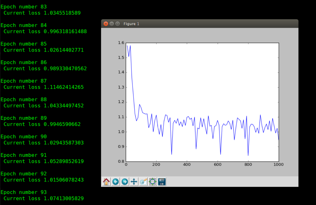
     y_tr = np.zeros(BATCH_SIZE).astype('int32')

     for epoch in range(NUM_EPOCHS):
         batch_train_losses = []
         pbar = ProgressBar(widgets=widgets, maxval=num_batches).start()
         for k in range(num_batches):
             sh = shuf[k*BATCH_SIZE:k*BATCH_SIZE+BATCH_SIZE]
             pbar.update(k)
             # fill batch here
             for s in range(0,BATCH_SIZE*2,2):
                 # idx1 = dtrain['traingt'][sh[s/2],0]
                 # idx2 = dtrain['traingt'][sh[s/2],1]
                 # lbl = dtrain['traingt'][sh[s/2],2]

                 idx1 = dtr[sh[s/2]][0]
                 idx2 = dtr[sh[s/2]][1]
                 lbl = dtr[sh[s/2]][2]

                 X_tr[s] = dtrain['patches'][idx1]
                 X_tr[s+1] = dtrain['patches'][idx2]
                 y_tr[s/2] = lbl

             batch_train_loss = trainf(X_tr,y_tr)
             batch_train_losses.append(batch_train_loss)
         avg_train_loss = np.mean(batch_train_losses)
         pbar.finish()
         print("> Epoch " + str(epoch) + ", loss: "+str(avg_train_loss))

         eval_test(net,dtest)

         with open('net.pickle', 'wb') as f:
             pickle.dump(net, f, -1)

         # netlayers = lasagne.layers.get_all_layers(net)
         # print(netlayers)
         # layer = netlayers[1]
         # print(layer)
         # print(layer.num_filters)
         # W = layer.W.get_value()
         # b = layer.b.get_value()
         # f = [w + bb for w, bb in zip(W, b)]
         # gs = gridspec.GridSpec(8, 12)
         # for i in range(layer.num_filters):
         #     g = gs[i]
         #     ax = plt.subplot(g)
         #     ax.grid()
         #     ax.set_xticks([])
         #     ax.set_yticks([])
         #     ax.imshow(f[i][0])
         # plt.show()

 if __name__ == '__main__':
    main(sys.argv[1])

3. Tensorflow version :

Github link: https://github.com/ywpkwon/siamese_tf_mnist

4. PyTorch Version: 

Github link: https://github.com/harveyslash/Facial-Similarity-with-Siamese-Networks-in-Pytorch/blob/master/Siamese-networks-medium.ipynb

5.