Link Analysis_1_Basic Elements

1. Edge Attributes

1.1 Methods of category

1.1.1 Basic three categories in terms of number of layers as edges or direction of edges:

import networkx as nx
G = nx.DiGraph() # 1.directed
G = nx.Graph() # 2.undirected
G = nx.MultiGraph() # 3.between two nodes many layers of relationships

1.1.2 Logical categories in terms of cluster characteristics, i.e., Bipartite:

from networkx.algorithms import bipartite
B = nx.Graph() # create an empty network first step, no subsets of nodes
B.add_nodes_from(['H', 'I', 'J', 'K', 'L'], bipartite = 0) # label 1 group
B.add_nodes_from([7, 8, 9, 10], bipartite = 1) # label 2

# add a list of edges at one time
B.add_edges_from([('H', 7), ('I', 7), ('J', 9),('K', 8), ('K', 10), ('L', 10)])
# Chect if bipartite or not
bipartite.is_bipartite(B)

Bipartite graph cannot contain a cycle of an odd number of nodes.

1.2 Edge can contain detailed features:

G.add_edge('A', 'B', weight = 6, relation = 'family', sign = '+')
G.remove_edge('A', 'B') # remove edge

1.3 Access edges:

G.edges() # list of all edges
G.edges(data = True) # list of all with attributes
G.edges(data = 'relation') # list with certain attribute

2. Node Attributes

2.1 Node be named as character.

G.add_node('A', name = 'Sophie')
G.add_node('B', name = 'Cumberbatch')
G.add_node('C', name = 'Miko') # pet dog

2.2 Access nodes:

G.node['A']['name']

3. Network Connectivity

3.1 Triadic Closure: Tendency for people who have shared connections to become connects, i.e., to cluster.

3.1.1 Local Clustering Coefficient

# local clustering only for multigraph type
G = nx.Graph()
G.add_edges_from([('A', 'K'),
                 ('A', 'B'),
                 ('A', 'C'),
                 ('B', 'C'),
                 ('B', 'K'),
                 ('C', 'E'),
                 ('C', 'F'),
                 ('D', 'E'),
                 ('E', 'F'),
                 ('E', 'H'),
                 ('F', 'G'),
                 ('I', 'J')])
nx.clustering(G, 'A')

0.6666666666666666

Solve: 2 / [2 × 3 ÷ 2] # actual pairs / (C32)

3.1.2 Global Clustering Coefficient

# Method 1: Take average of all local clustering coefficients.
nx.average_clustering(G)

0.28787878787878785

# Method 2: Percent of open triads that are triangles in the network
# Triange: 3 nodes connected by 3 edges
# open triads: 3 nodes connected by 2 edges
# Transitivity = (3 * number of closed triads) / number of open triads
nx.transitivity(G)

0.4090909090909091

Method 2 put a larger weight on high degree nodes.

3.2 Distances

3.2.1 Singe Pair Pattern:

Find path and length of the shortest path between two nodes.

nx.shortest_path(G, 'A', 'H')

['A', 'C', 'E', 'H']

nx.shortest_path_length(G, 'A', 'H')

3

3.2.2 One Node to Every Others Pattern:

Breadth-first Search: discover nodes in layers step by step.

T = nx.bfs_tree(G, 'A')
T.edges() # to get the tree

OutEdgeView([('A', 'K'), ('A', 'B'), ('A', 'C'), ('C', 'E'), ('C', 'F'), ('E', 'D'), ('E', 'H'), ('F', 'G')])

nx.shortest_path_length(G, 'A') # get dictionary of distances from A to others

{'A': 0, 'K': 1, 'B': 1, 'C': 1, 'E': 2, 'F': 2, 'D': 3, 'H': 3, 'G': 3}

3.2.3 Measures of Distance Patterns

# Average of all
nx.average_shortest_path_length(G)
# Maximum distance
nx.diameter(G)

Eccentricity of a node is the largest distance between A and all others.

Radius is the minimum eccentricity.

Periphery is the set of nodes that have eccentricity equal to the diameter.

Center is the set of nodes with eccentricity equal to radius.

nx.eccentricity(G)
nx.radius(G)
nx.periphery(G)
nx.center(G)

3.2.4 Application

import numpy as np
import pandas as pd
%matplotlib notebook
# Instantiate the graph
G = nx.karate_club_graph()
nx.draw_networkx(G)

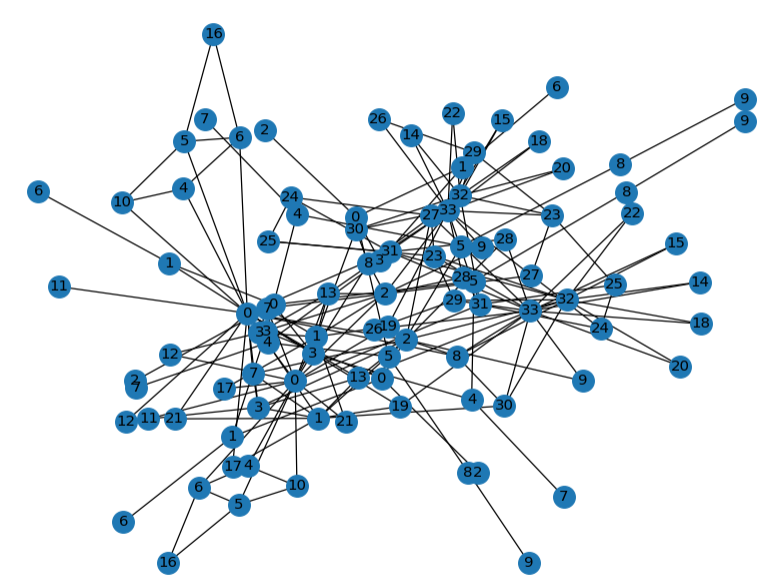
4. Connectivity

4.1 Connectivity in Undirected Graphs

# find number of communities (connected componets)
nx.number_connected_componets(G)
# give list of them
sorted(nx.connected_components(G))
# find the community to which 'M' belongs
nx.node_connected_components(G, 'M')

4.2 Connectivity in Directed Graphs

# find strongly connected component (directed path to every other nodes &
# no other node has directed path to this subset)
sorted(nx_strongly_connected_components(G))

5. Network Robustness

5.1 Definition: the ability for network to maintain general structural properties (connectivity) when faced with attacks (removal of edges or nodes).

# smallest number of nodes needed to disconnect
nx.node_connectivity(G_un)
# which nodes
nx.minimum_code_cut(G_un)
# smallest number of edges needed to disconnect
nx.edge_connectivity(G_un)
# which edges
nx.minimum_edge_cut(G_un)

5.2 Node Connectivity

# ways to deliver msg from 'G' to 'L'
sorted(nx.all_simple_paths(G, 'G', 'L'))
# want to block this path, how many nodes neeed to remove
nx.node_connectivity(G, 'G', 'L')
# which nodes
nx.minimum_node_cut(G, 'G', 'L')

5.3 Edge Connectivity

# how many
nx.edge_connectivity(G, 'G', 'L')
# show in details
nx.minimum_edge_cut(G, 'G', 'L')

6. Centrality

6.1 Degree Centrality

6.1.1 Undirected Network

G = nx.karate_club_graph()
G = nx.convert_node_labels_to_integers(G, first_label = 1)
degCent = nx.degree_centrality(G)

degCent[34]

0.5151515151515151

6.1.2 Directed Network

indegCent = nx.in_degree_centrality(G)

indegCent = nx.out_degree_centrality(G)

6.2 Closeness Centrality

6.2.1 Calculation: Shorter distance away from all other nodes.

closeCent = nx.closeness_centrality(G)
closeCent[34]

0.55

sum(nx.shortest_path_length(G, 34).values())

60

# Essence is equivalent to process below
(len(G.nodes()) - 1)/61

0.5409836065573771

6.2.2 Disconnceted Nodes Measurement

Method One

# choose non-normalizing, closeness centrality would be one
nx.closeness_centrality(G, normalized = False)

1

Method Two

# choose normalising,i.e. divide by (total nodes - 1)
nx.closeness_centrality(G, normalized = True)

0.071

6.3 Betweenness Centrality (computationally expensive)

Essence: Find nodes which shows up in many shortest paths between two nodes.

6.3.1 Method One: Use all 34 nodes in karate club

btwnCent = nx.betweenness_centrality(G,normalized = True, endpoints = False)
import operator
sorted(btwnCent.items(), key = operator.itemgetter(1), reverse = True)[0:5]

[(1, 0.43763528138528146),
 (34, 0.30407497594997596),
 (33, 0.145247113997114),
 (3, 0.14365680615680618),
 (32, 0.13827561327561325)]

6.3.2 Method Two: Use 10 nodes as approximation

btwnCent_approx = nx.betweenness_centrality(G,normalized = True, endpoints = False, k = 10)
sorted(btwnCent_approx.items(), key = operator.itemgetter(1), reverse = True)[0:5]

[(1, 0.3674031986531986),
 (34, 0.3048388648388649),
 (32, 0.17290028258778256),
 (3, 0.13572044853294854),
 (33, 0.130249518999519)]

6.3.3 Method Three: Specify subsets

btwnCent_subset = nx.betweenness_centrality_subset(G,
                                                  [34, 33, 21, 30, 16, 27, 15, 23, 10],
                                                  [1, 4, 13, 11, 6, 12, 17, 7],
                                                  normalized = True)
sorted(btwnCent_subset.items(), key = operator.itemgetter(1), reverse = True)[0:5]

[(1, 0.04899515993265994),
 (34, 0.028807419432419434),
 (3, 0.018368205868205867),
 (33, 0.01664712602212602),
 (9, 0.014519450456950456)]

6.3.4 Method Four: Edges

btwnCent_edge = nx.edge_betweenness_centrality(G, normalized = True)
sorted(btwnCent_edge.items(), key = operator.itemgetter(1), reverse = True)[0:5]
# node 1 is the instructor of club

[((1, 32), 0.1272599949070537),
 ((1, 7), 0.07813428401663695),
 ((1, 6), 0.07813428401663694),
 ((1, 3), 0.0777876807288572),
 ((1, 9), 0.07423959482783014)]

btwnCent_edge_subset = nx.edge_betweenness_centrality_subset(G,
                                                            [34, 33, 21, 30, 16, 27, 15, 23, 10],
                                                              [1, 4, 13, 11, 6, 12, 17, 7],
                                                             normalized = True)
sorted(btwnCent_edge_subset.items(), key = operator.itemgetter(1), reverse = True)[0:5]

[((1, 9), 0.01366536513595337),
 ((1, 32), 0.01366536513595337),
 ((14, 34), 0.012207509266332794),
 ((1, 3), 0.01211343123107829),
 ((1, 6), 0.012032085561497326)]