Matlab实现线性回归和逻辑回归: Linear Regression & Logistic Regression

原文：http://blog.csdn.net/abcjennifer/article/details/7732417

本文为Maching Learning 栏目补充内容，为上几章中所提到单参数线性回归、多参数线性回归和 逻辑回归的总结版。旨在帮助大家更好地理解回归，所以我在Matlab中分别对他们予以实现，在本文中由易到难地逐个介绍。

 

 

本讲内容：

Matlab 实现各种回归函数

=========================

基本模型

Y=θ₀+θ₁X₁型---线性回归（直线拟合）

解决过拟合问题---Regularization

Y=1/(1+e^X)型---逻辑回归（sigmod 函数拟合）

=========================

 

第一部分：基本模型

 

在解决拟合问题的解决之前，我们首先回忆一下线性回归和逻辑回归的基本模型。

设待拟合参数 θ_n*1 和输入参数[ x_m*n, y_m*1 ] 。

对于各类拟合我们都要根据梯度下降的算法，给出两部分：

①   cost function（指出真实值y与拟合值h<hypothesis>之间的距离）：给出cost function 的表达式，每次迭代保证cost function的量减小；给出梯度gradient，即cost function对每一个参数θ的求导结果。

function [ jVal,gradient ] = costFunction ( theta )

②   Gradient_descent（主函数）：用来运行梯度下降算法，调用上面的cost function进行不断迭代，直到最大迭代次数达到给定标准或者cost function返回值不再减小。

function [optTheta,functionVal,exitFlag]=Gradient_descent( )

线性回归：拟合方程为h_θ(x)=θ₀x₀+θ₁x₁+…+θ_nx_n，当然也可以有x_n的幂次方作为线性回归项（如），这与普通意义上的线性不同，而是类似多项式的概念。

其cost function 为：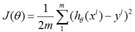

逻辑回归：拟合方程为h_θ(x)=1/(1+e^(θ^Tx))，其cost function 为：

cost function对各θj的求导请自行求取，看第三章最后一图，或者参见后文代码。

_{后面，我们分别对几个模型方程进行拟合，给出代码，并用matlab中的fit函数进行验证。}

 

 

第二部分：Y=θ₀+θ₁X₁型---线性回归（直线拟合）

 

在Matlab 线性拟合 & 非线性拟合中我们已经讲过如何用matlab自带函数fit进行直线和曲线的拟合，非常实用。而这里我们是进行ML课程的学习，因此研究如何利用前面讲到的梯度下降法（gradient descent）进行拟合。

cost function：

 function [ jVal,gradient ] = costFunction2( theta )
 %COSTFUNCTION2 Summary of this function goes here
 %   linear regression -> y=theta0 + theta1*x
 %   parameter: x:m*n  theta:n*   y:m*   (m=,n=)
 %   

 %Data
 x=[;;;];
 y=[1.1;2.2;2.7;3.8];
 m=size(x,);

 hypothesis = h_func(x,theta);
 delta = hypothesis - y;
 jVal=sum(delta.^);

 gradient()=sum(delta)/m;
 gradient()=sum(delta.*x)/m;

 end

其中，h_func是hypothesis的结果：

 function [res] = h_func(inputx,theta)
 %H_FUNC Summary of this function goes here
 %   Detailed explanation goes here

 %cost function
 res= theta()+theta()*inputx;function [res] = h_func(inputx,theta)
 end

Gradient_descent：

 function [optTheta,functionVal,exitFlag]=Gradient_descent( )
 %GRADIENT_DESCENT Summary of this function goes here
 %   Detailed explanation goes here

   options = optimset('GradObj','on','MaxIter',);
   initialTheta = zeros(,);
   [optTheta,functionVal,exitFlag] = fminunc(@costFunction2,initialTheta,options);

 end

result：

 >> [optTheta,functionVal,exitFlag] = Gradient_descent()

 Local minimum found.

 Optimization completed because the size of the gradient is less than
 the default value of the function tolerance.

 <stopping criteria details>

 optTheta =

     0.3000
     0.8600

 functionVal =

     0.0720

 exitFlag =

即得y=0.3+0.86x;

验证：

 function [ parameter ] = checkcostfunc(  )
 %CHECKC2 Summary of this function goes here
 %   check if the cost function works well
 %   check with the matlab fit function as standard

 %check cost function
 x=[;;;];
 y=[1.1;2.2;2.7;3.8];

 EXPR= {'x',''};
 p=fittype(EXPR);
 parameter=fit(x,y,p);

 end

运行结果：

 >> checkcostfunc()

 ans = 

      Linear model:
      ans(x) = a*x + b
      Coefficients (with % confidence bounds):
        a =        0.86  (0.4949, 1.225)
        b =         0.3  (-0.6998, 1.3)

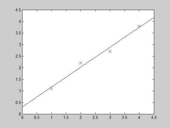
和我们的结果一样。下面画图：

 function PlotFunc( xstart,xend )
 %PLOTFUNC Summary of this function goes here
 %   draw original data and the fitted 

 %===================cost function ====linear regression
 %original data
 x1=[;;;];
 y1=[1.1;2.2;2.7;3.8];
 %plot(x1,y1,'ro-','MarkerSize',);
 plot(x1,y1,'rx','MarkerSize',);
 hold on;

 %fitted line - 拟合曲线
 x_co=xstart:0.1:xend;
 y_co=0.3+0.86*x_co;
 %plot(x_co,y_co,'g');
 plot(x_co,y_co);

 hold off;
 end

 

 

第三部分：解决过拟合问题---Regularization

 

过拟合问题解决方法我们已在第三章中讲过，利用Regularization的方法就是在cost function中加入关于θ的项，使得部分θ的值偏小，从而达到fit效果。

例如定义costfunction J(θ)： jVal=(theta(1)-5)^2+(theta(2)-5)^2;

在每次迭代中，按照gradient descent的方法更新参数θ：θ(i)-=gradient(i),其中gradient(i)是J(θ)对θi求导的函数式，在此例中就有gradient(1)=2*(theta(1)-5), gradient(2)=2*(theta(2)-5)。

函数costFunction, 定义jVal=J(θ)和对两个θ的gradient：

 function [ jVal,gradient ] = costFunction( theta )
 %COSTFUNCTION Summary of this function goes here
 %   Detailed explanation goes here

 jVal= (theta()-)^+(theta()-)^;

 gradient = zeros(,);
 %code to compute derivative to theta
 gradient() =  * (theta()-);
 gradient() =  * (theta()-);

 end

Gradient_descent，进行参数优化

 function [optTheta,functionVal,exitFlag]=Gradient_descent( )
 %GRADIENT_DESCENT Summary of this function goes here
 %   Detailed explanation goes here

  options = optimset('GradObj','on','MaxIter',);
  initialTheta = zeros(,)
  [optTheta,functionVal,exitFlag] = fminunc(@costFunction,initialTheta,options);

 end

matlab主窗口中调用，得到优化厚的参数(θ1,θ2)=(5,5)

  [optTheta,functionVal,exitFlag] = Gradient_descent()

 initialTheta =

 Local minimum found.

 Optimization completed because the size of the gradient is less than
 the default value of the function tolerance.

 <stopping criteria details>

 optTheta =

 functionVal =

 exitFlag =

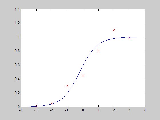
第四部分：Y=1/(1+e^X)型---逻辑回归（sigmod 函数拟合）

hypothesis function:

 function [res] = h_func(inputx,theta)

 %cost function
 tmp=theta()+theta()*inputx;%m*
 res=./(+exp(-tmp));%m*

 end

cost function:

 function [ jVal,gradient ] = costFunction3( theta )
 %COSTFUNCTION3 Summary of this function goes here
 %   Logistic Regression

 x=[-;      -;     -;     ;      ;      ;     ];
 y=[0.01;    0.05;   0.3;    0.45;   0.8;    1.1;    0.99];
 m=size(x,);

 %hypothesis  data
 hypothesis = h_func(x,theta);

 %jVal-cost function  &  gradient updating
 jVal=-sum(log(hypothesis+0.01).*y + (-y).*log(-hypothesis+0.01))/m;
 gradient()=sum(hypothesis-y)/m;   %reflect to theta1
 gradient()=sum((hypothesis-y).*x)/m;    %reflect to theta 

 end

Gradient_descent:

 function [optTheta,functionVal,exitFlag]=Gradient_descent( )

  options = optimset('GradObj','on','MaxIter',);
  initialTheta = [;];
  [optTheta,functionVal,exitFlag] = fminunc(@costFunction3,initialTheta,options);

 end

运行结果：

  [optTheta,functionVal,exitFlag] = Gradient_descent()

 Local minimum found.

 Optimization completed because the size of the gradient is less than
 the default value of the function tolerance.

 <stopping criteria details>

 optTheta =

     0.3526
     1.7573

 functionVal =

     0.2498

 exitFlag =

 

画图验证：

 

 

 

有朋友问，这里就补充一下logistic regression中gradient的推导：

令

则有

由于cost function

可得

所以gradient = -J'(theta) = (z-y)x