有限元方法[Matlab]-笔记

<< MATLAB Codes for Finite Element Analysis - Solids and Structures (Ferreira) >> 笔记
第一章:matlab基础
略
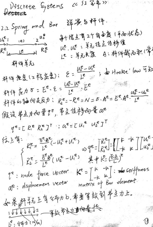
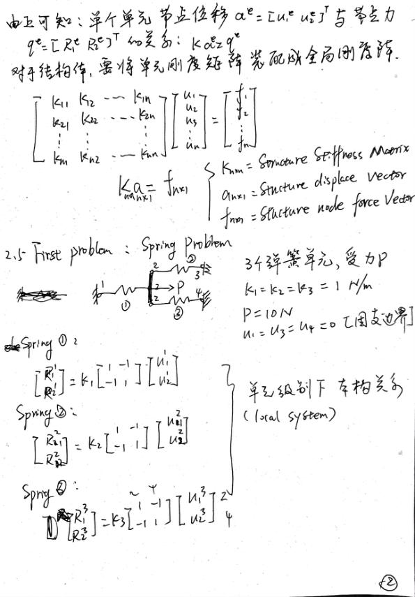
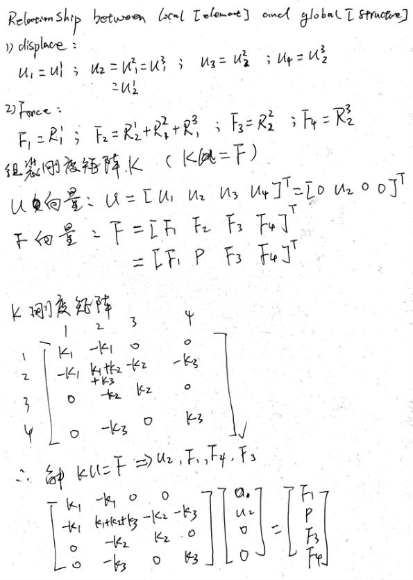
第二章: 离散系统
笔记、例题
Matlab代码
problem1.m
% MATLAB codes for Finite Element Analysis

%  Problem 1: 3 springs problem

% clear memory

clear ;

% ? define vars

P=10; % N

ki=[1;1;1;1];

% elementNodes: connections at elements

elementNodes=[1 2;

            2 3;

            2 4];

% numberElements: number of Elements

numberElements=size(elementNodes,1);

% numberNodes: number of nodes

numberNodes=4;

% for structure:

% displacements: displacement vector N x 1

% force : force vector N x 1

% stiffness: stiffness matrix N x N

displacements=zeros(numberNodes,1); %#ok<PREALL>

force=zeros(numberNodes,1);

stiffness=zeros(numberNodes);

% applied load at node 2

force(2)=P;

% computation of the system stiffness matrix

for e=1:numberElements

    % elementDof: element degrees of freedom (Dof)

    elementDof=elementNodes(e,:) ;

    stiffness(elementDof,elementDof)=...

    stiffness(elementDof,elementDof)+ki(e)*[1 -1;-1 1];

end

% boundary conditions and solution

% prescribed dofs

prescribedDof=[1;3;4];

% free Dof : activeDof

% setdiff() 函数-->求两个数组的差集

% C = setdiff(A,B) 返回 A 中存在但 B 中不存在的数据,不包含重复项.C 是有序的.

activeDof=setdiff((1:numberNodes)',prescribedDof);

% solution

% !KU=F --> U=K\F

displacements=stiffness(activeDof,activeDof)\force(activeDof);

% positioning all displacements

displacements1=zeros(numberNodes,1);

displacements1(activeDof)=displacements;

% output displacements/reactions

outputDisplacementsReactions(displacements1,stiffness,numberNodes,prescribedDof)
outputDisplacementsReactions.m
function outputDisplacementsReactions(displacements,stiffness,GDof,prescribedDof)

    % output of displacements and reactions in

    % tabular form

    % GDof: total number of degrees of freedom of the problem

    % displacements

    disp('Displacements')

    %displacements=displacements1;

    jj=1:GDof; % format

    [jj' displacements]

    % reactions

    F=stiffness*displacements;

    reactions=F(prescribedDof);

    disp('reactions')

    [prescribedDof reactions]

end
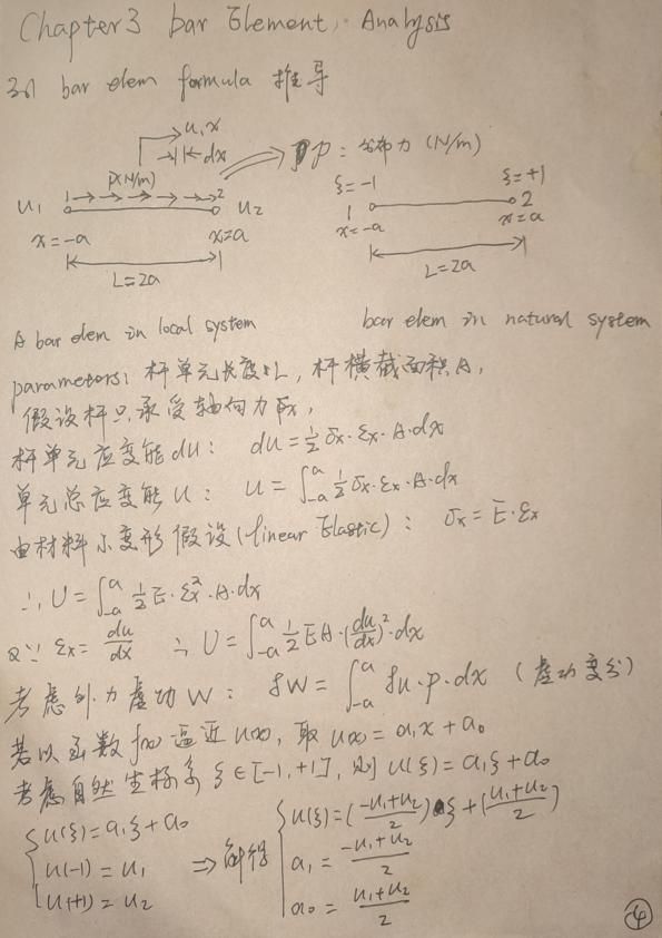
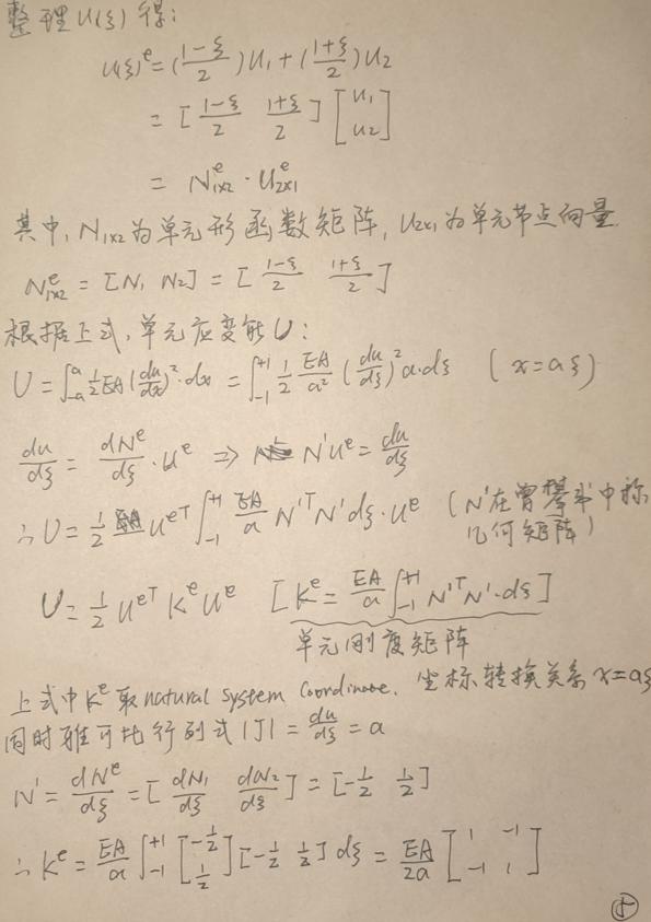
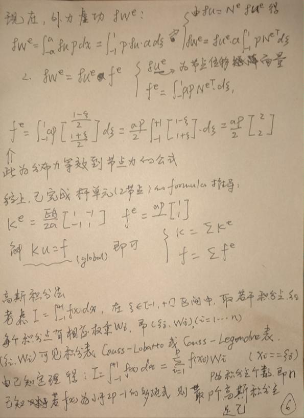
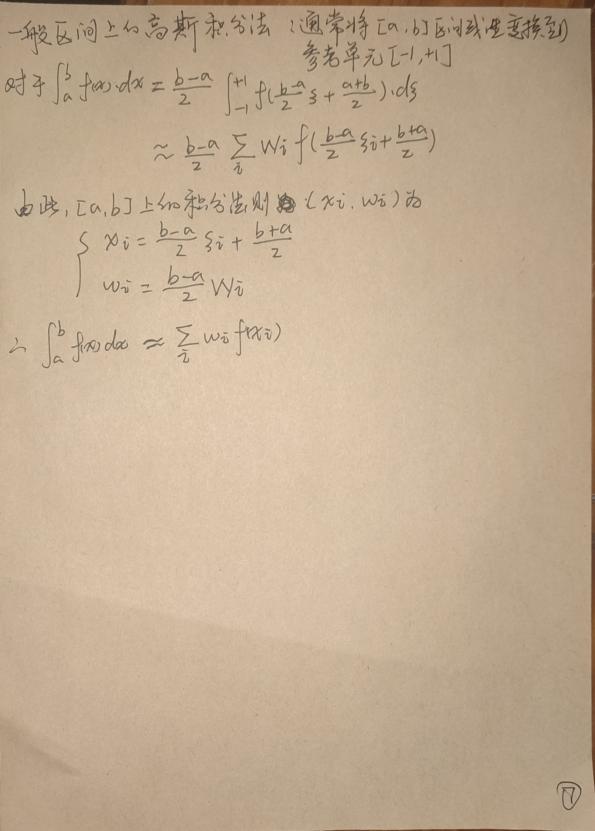
第三章:1D 杆单元
笔记
例题1
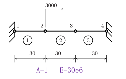

matlab 代码
problem2.m
% antonio ferreira 2008

% clear memory

clear all

% E; modulus of elasticity

% A: area of cross section

% L: length of bar

E = 30e6;A=1;EA=E*A; L = 90;

% generation of coordinates and connectivities

% numberElements: number of elements

numberElements=3;

% generation equal spaced coordinates

nodeCoordinates=linspace(0,L,numberElements+1);

xx=nodeCoordinates;

% numberNodes: number of nodes

numberNodes=size(nodeCoordinates,2);

% elementNodes: connections at elements

ii=1:numberElements;

elementNodes(:,1)=ii;

elementNodes(:,2)=ii+1;

% for structure:

% displacements: displacement vector

% force : force vector

% stiffness: stiffness matrix

displacements=zeros(numberNodes,1); %#ok<PREALL>

force=zeros(numberNodes,1);

stiffness=zeros(numberNodes,numberNodes);

% applied load at node 2

force(2)=3000.0;

% computation of the system stiffness matrix

for e=1:numberElements;

    % elementDof: element degrees of freedom (Dof)

    elementDof=elementNodes(e,:) ;

    nn=length(elementDof);

    length_element=nodeCoordinates(elementDof(2))...

    -nodeCoordinates(elementDof(1));

    detJacobian=length_element/2;invJacobian=1/detJacobian;

    % central Gauss point (xi=0, weight W=2)

    [shape,naturalDerivatives]=shapeFunctionL2(0.0);

    Xderivatives=naturalDerivatives*invJacobian;

    % B matrix

    B=zeros(1,nn); B(1:nn) = Xderivatives(:);

    stiffness(elementDof,elementDof)=stiffness(elementDof,elementDof)+B'*B*2*detJacobian*EA;

end

% boundary conditions and solution

% prescribed dofs

fixedDof=find(xx==min(nodeCoordinates(:)) | xx==max(nodeCoordinates(:)))';

prescribedDof=[fixedDof]

% free Dof : activeDof

activeDof=setdiff([1:numberNodes]',[prescribedDof]);

% solution

GDof=numberNodes;

displacements=solution(GDof,prescribedDof,stiffness,force);

% output displacements/reactions

outputDisplacementsReactions(displacements,stiffness,numberNodes,prescribedDof)

disp(stiffness)

disp(force)

disp(displacements)
solution.m
function displacements=solution(GDof,prescribedDof,stiffness,force)

    % function to find solution in terms of global displacements

    activeDof=setdiff([1:GDof]', ...

    [prescribedDof]);

    U=stiffness(activeDof,activeDof)\force(activeDof);

    displacements=zeros(GDof,1);

    displacements(activeDof)=U;

end
shapeFunctionL2.m
function [shape,naturalDerivatives]=shapeFunctionL2(xi)

    % shape function and derivatives for L2 elements

    % shape : Shape functions

    % naturalDerivatives: derivatives w.r.t. xi

    % xi: natural coordinates (-1 ... +1)

    shape=([1-xi,1+xi]/2)';

    naturalDerivatives=[-1;1]/2;

end
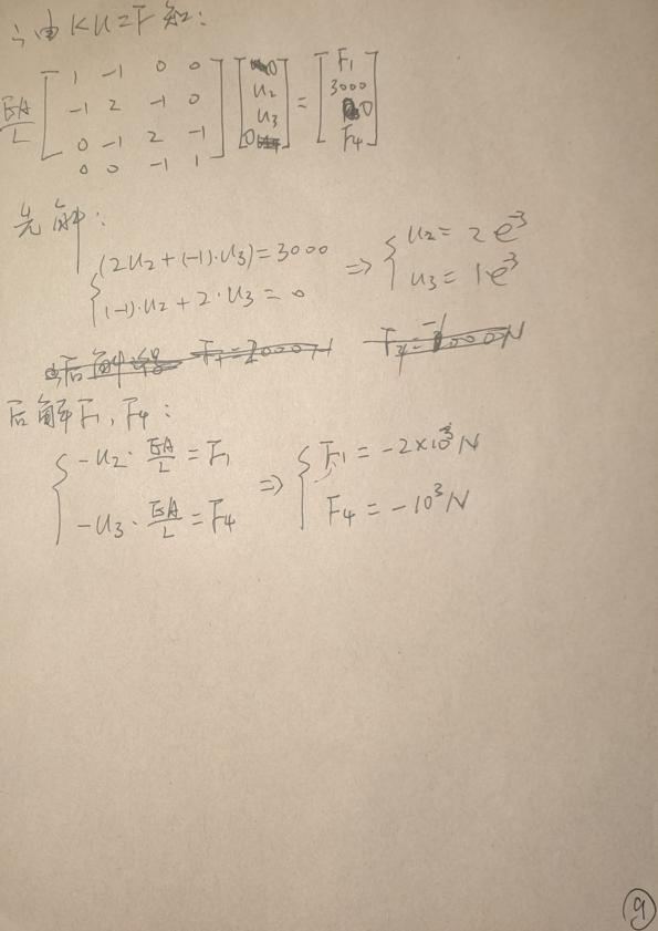
例题2
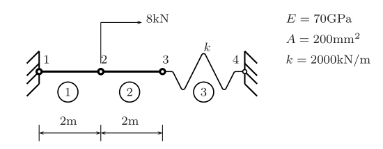
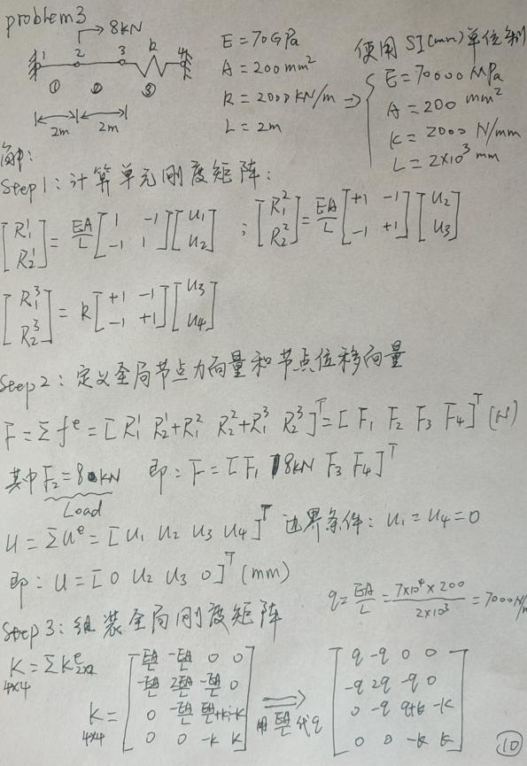
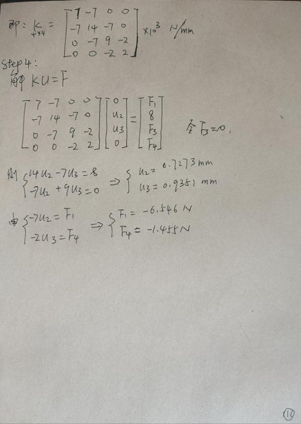
matlab 代码
problem3Structure.m
% MATLAB codes for Finite Element Analysis

% antonio ferreira 2008

% clear memory

clear all

% p1 : structure

p1=struct();

% E; modulus of elasticity

% A: area of cross section

% L: length of bar

% k: spring stiffness

E=70000;

A=200;

k=2000;

% generation of coordinates and connectivities

% numberElements: number of elements

p1.numberElements=3;

p1.numberNodes=4;

p1.elementNodes=[1 2; 2 3; 3 4];

p1.nodeCoordinates=[0 2000 4000 4000];

p1.xx=p1.nodeCoordinates;

% GDof: total degrees of freedom

p1.GDof=p1.numberNodes;

% for structure:

    % displacements: displacement vector

    % force : force vector

    % stiffness: stiffness matrix

p1.displacements=zeros(p1.GDof,1);

p1.force=zeros(p1.GDof,1);

p1.stiffness=zeros(p1.GDof);

% applied load at node 2

p1.force(2)=8000.0;

% computation of the system stiffness matrix

for e=1:p1.numberElements;

    % elementDof: element degrees of freedom (Dof)

    elementDof=p1.elementNodes(e,:) ;

    L=p1.nodeCoordinates(elementDof(2))-p1.nodeCoordinates(elementDof(1));

    if e<3

        ea(e)=E*A/L;

    else

        ea(e)=k;

    end

    p1.stiffness(elementDof,elementDof)=p1.stiffness(elementDof,elementDof)+ea(e)*[1 -1;-1 1];

end

% prescribed dofs

p1.prescribedDof=[1;4];

% solution

p1.displacements=solutionStructure(p1);

% output displacements/reactions

outputDisplacementsReactionsStructure(p1)

% Displacements

% ans =

%     1.0000         0

%     2.0000    3.3333

%     3.0000         0

%     4.0000         0

% reactions

% ans =

%     1.0000   -3.3333

%     3.0000   -3.3333

%     4.0000   -3.3333
outputDisplacementsReactionsStructure.m
function outputDisplacementsReactionsStructure(p)

    % output of displacements and reactions in

    % tabular form

    % GDof: total number of degrees of freedom of

    % the problem

    % displacements

    disp('Displacements')

    jj=1:p.GDof;

    [jj' p.displacements]

    % reactions

    F=p.stiffness*p.displacements;

    reactions=F(p.prescribedDof);

    disp('reactions')

    [p.prescribedDof reactions]
shapeFunctionL2Structure.m
function shapeL2=shapeFunctionL2Structure(xi)

    % shape function and derivatives for L2 elements

    % shape : Shape functions

    % naturalDerivatives: derivatives w.r.t. xi

    % xi: natural coordinates (-1 ... +1)

    shapeL2=struct()

    shapeL2.shape=([1-xi,1+xi]/2)';

    shapeL2.naturalDerivatives=[-1;1]/2;

end % end function shapeFunctionL2
solutionStructure.m
function displacements = solutionStructure(p)

    % function to find solution in terms of global displacements

    activeDof=setdiff([1:p.GDof]', [p.prescribedDof]);

    U=p.stiffness(activeDof,activeDof)\p.force(activeDof);

    displacements=zeros(p.GDof,1);

    displacements(activeDof)=U;

end
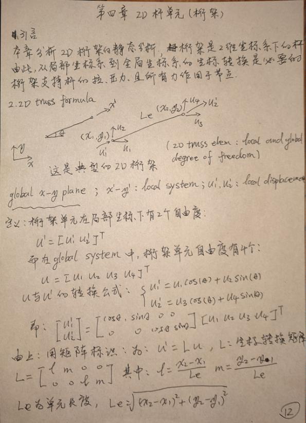
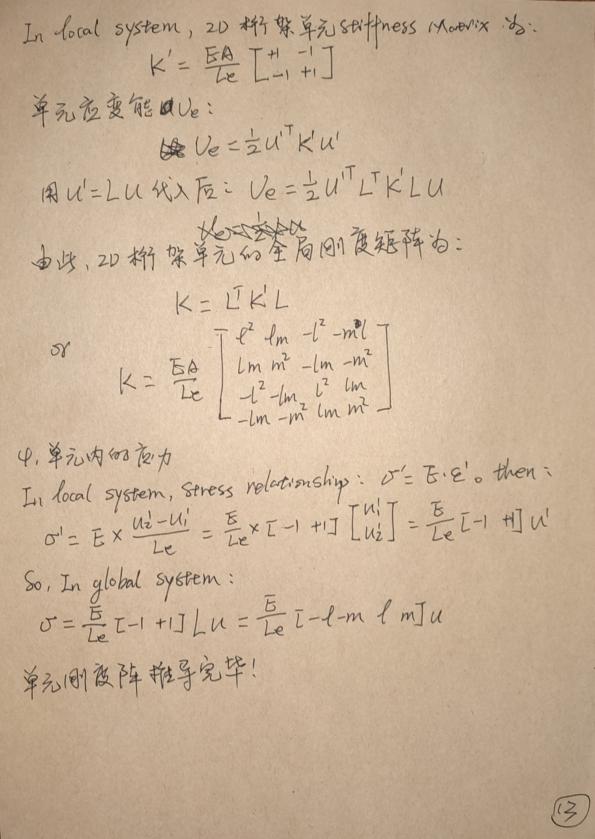
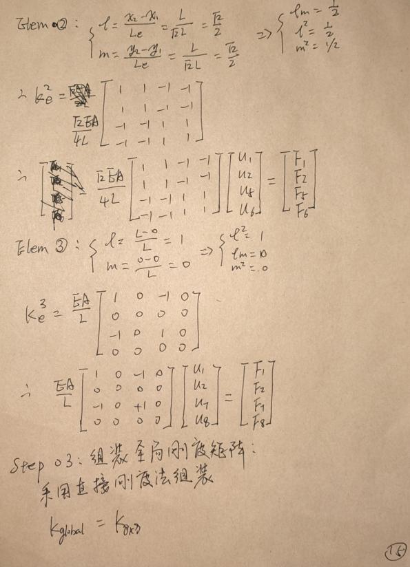
第四章 2D桁架分析
笔记:单元刚度矩阵推导
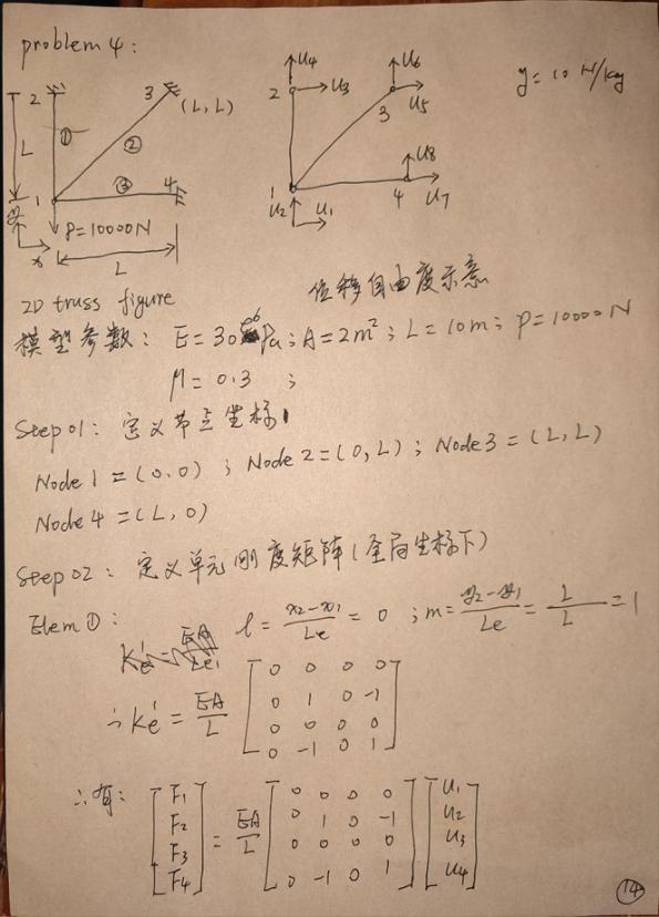
例题1
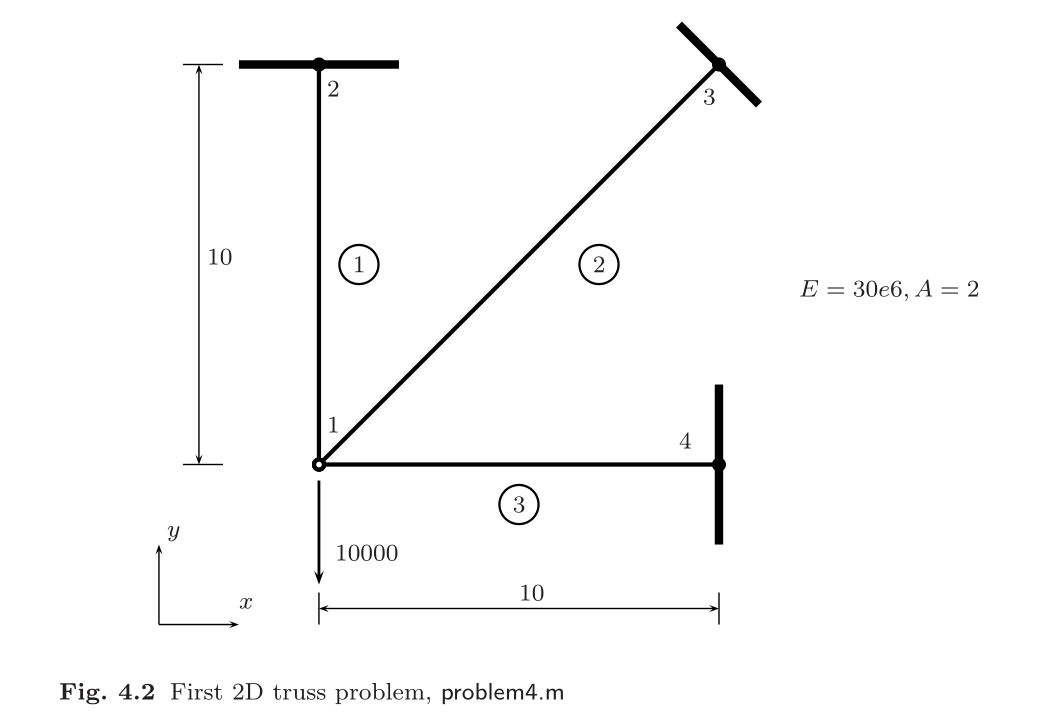
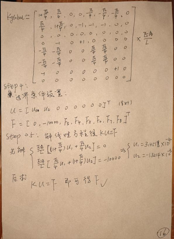
模型参数:
- 杨氏模量E=30e6 Pa ,泊松比 \(\mu\) =0.3
- A=2 m^2
- L=10 m
- P=10000 N
手算过程
Abaqus 模拟结果
inp文件在码云repo中
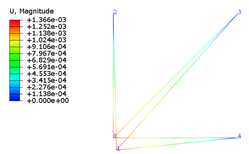
U and RF result :
********************************************************************************

Probe Values Report, written on Tue Apr 16 21:43:02 2024

Source

-------

   ODB: C:/Users/Administrator/Documents/learnFEM/Matlb Fea Codes repo/fea-codes-of-matlab/chapter04/problem4/abaqus/Job-2.odb

   Step: Step-1

   Frame: Increment      1: Step Time =    1.000

   Variable: U, U1

Probe values reported at nodes

  Part Instance     Node ID                   Orig. Coords                                     Def. Coords

                                    X               Y               Z               X               Y               Z

-------------------------------------------------------------------------------------------------------------------------

    PART-1-1           1              0.              0.              0.     345.178E-06    -1.32149E-03              0.

    PART-1-1           2              0.             10.              0.              0.             10.              0.

    PART-1-1           3             10.             10.              0.             10.             10.              0.

    PART-1-1           4             10.              0.              0.             10.              0.              0.

  Part Instance     Node ID  Attached elem      U, U1        U, U2           RF, RF1         RF, RF2

--------------------------------------------------------------------------------------------------------------

    PART-1-1           1         3          345.178E-06    -1.32149E-03              0.              0.

    PART-1-1           2         1                   0.    -7.92893E-33              0.     7.92893E+03

    PART-1-1           3         2         -2.07107E-33    -2.07107E-33     2.07107E+03     2.07107E+03

    PART-1-1           4         3          2.07107E-33              0.    -2.07107E+03             -0.
可以看出,手算和abaqus的U结果完全一致.
matlab 代码
problem4.m
% ! problem4.m --> based on <<MATLAB codes for Finite Element Analysis>>

clear ;

clc

format default

p=struct();

% define model parameters

p.E = 30e6;

p.A = 2;

p.L = 10;

p.P = -10000;

% define elems and nodes

p.nodes=[0 0 ;  % node's coordinates (x,y)

         0 p.L ;

         p.L p.L ;

         p.L 0 ];

p.elems=[1 2 ;

        1 3 ;

        1 4];

p.node_num=size(p.nodes,1);

p.elem_num=size(p.elems,1);

p.node_Coord_x=p.nodes(:,1);

p.node_Coord_y=p.nodes(:,2);

% define problem's dimension : 1D/2D/3D;

%        = each node's dof

p.problem_dimension=size(p.nodes,2);

% global degree of freedom number

p.global_dof_num=2*p.node_num;

% define global Nodal displacement  colum vector

p.displacements=zeros(p.global_dof_num,1);

p.node_forces=zeros(p.global_dof_num,1);

% define boundary conditions

% fixed dof

p.fix_dof=[3 4 5 6 7 8]';

% load dof and amplitude

p.load_dof=2;

% initial global stiffness matrix

p.global_stiffness_matrix=zeros(p.global_dof_num);

% compute all ElemStiffnessMatrix and assembly stiff matrix

elem_global_dof_num=2*size(p.elems,2);

p.elemStiffs=zeros(elem_global_dof_num,elem_global_dof_num,p.elem_num);

for i=1:p.elem_num

    connectivity=p.elems(i,:);

    % elem's all dof : a 2d truss node has 2 node,each node have 2 dof,

    % i-th node --> U_(2*i-1) and U_(2*i) dof(displacement of node)

    elem_dof=[connectivity(1)*2-1 connectivity(1)*2 ...

             connectivity(2)*2-1 connectivity(2)*2];

    node1_x=p.node_Coord_x(connectivity(1));

    node1_y=p.node_Coord_y(connectivity(1));

    node2_x=p.node_Coord_x(connectivity(2));

    node2_y=p.node_Coord_y(connectivity(2));

    elem_length=sqrt((node1_x-node2_x).^2+(node1_y-node2_y).^2);

    l=(node2_x-node1_x)/elem_length;

    m=(node2_y-node1_y)/elem_length;

    k_e=(p.E*p.A/elem_length)*...

        [l*l l*m -l*l -l*m;

         l*m m*m -l*m -m*m;

        -l*l -l*m l*l l*m;

        -l*m -m*m l*m m*m];

    p.elemStiffs(:,:,i)=k_e;

    % assemble stiffness matrix

    p.global_stiffness_matrix(elem_dof,elem_dof)=...

        p.global_stiffness_matrix(elem_dof,elem_dof)+k_e;

end

% apply boundary condition

p.displacements(p.fix_dof)=0;

p.node_forces(p.load_dof)=p.P;

% solution KU=F

p = solutionStruct(p);

% show compute result

disp('displacements of dofs :')

disp([(1:p.global_dof_num)', p.displacements])

disp('forces of dofs :')

disp([(1:p.global_dof_num)',p.node_forces])

figure

axis equal

% plot undeformed mesh

draw_2Dtruss_mesh(p.nodes,p)

% plot deformed mesh

deformed_node_coordinate=cal_deformed_nodes(p,500.0);

draw_2Dtruss_mesh(deformed_node_coordinate,p)

title('位移变形')

grid on

function new_p=solutionStruct(p)

    % free dof in structure

    free_dof=setdiff((1:p.global_dof_num)',p.fix_dof);

    % solute the equation :KU=F --> U=K\F

    U=p.global_stiffness_matrix(free_dof,free_dof)\p.node_forces(free_dof);

    p.displacements(free_dof)=U;

    % displacements=zeros(p.global_dof_num,1);

    p.node_forces=p.global_stiffness_matrix*p.displacements;

    new_p=p;

end

function deformed_node_coordinate=cal_deformed_nodes(p,scale)

    % initial

    deformed_node_coordinate=p.nodes;

    if p.problem_dimension==2

        index1=1:2:p.global_dof_num;

        index2=2:2:p.global_dof_num;

        deformed_node_coordinate(:,1)=deformed_node_coordinate(:,1)+p.displacements(index1)*scale;

        deformed_node_coordinate(:,2)=deformed_node_coordinate(:,2)+p.displacements(index2)*scale;

    elseif p.problem_dimension==3

        index1=1:3:p.global_dof_num;

        index2=2:3:p.global_dof_num;

        index3=3:3:p.global_dof_num;

        deformed_node_coordinate(:,1)=deformed_node_coordinate(:,1)+p.displacements(index1);

        deformed_node_coordinate(:,2)=deformed_node_coordinate(:,2)+p.displacements(index2);

        deformed_node_coordinate(:,3)=deformed_node_coordinate(:,3)+p.displacements(index3);

    end

end

function draw_2Dtruss_mesh(nodes,p)

    xy=zeros(size(p.elems,2)*p.elem_num,p.problem_dimension);

    cur1=1;

    cur2=0;

    for i =1:p.elem_num

        connectivity=p.elems(i,:);

        attach_node_num=size(connectivity,2);

        cur1=cur2+1;

        cur2=cur2+attach_node_num;

        coord=zeros(attach_node_num,p.problem_dimension);

        for j=1:size(connectivity,2)

            coord(j,:)=nodes(connectivity(j),:);

        end

        xy(cur1:cur2,:)=coord;

    end

    line(xy(:,1),xy(:,2),"Marker","o","LineWidth",1,"Color",rand(1,3))

end
三种方式,计算结果一致
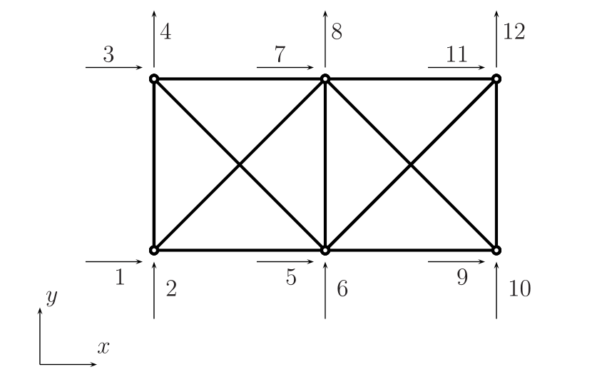
例题2
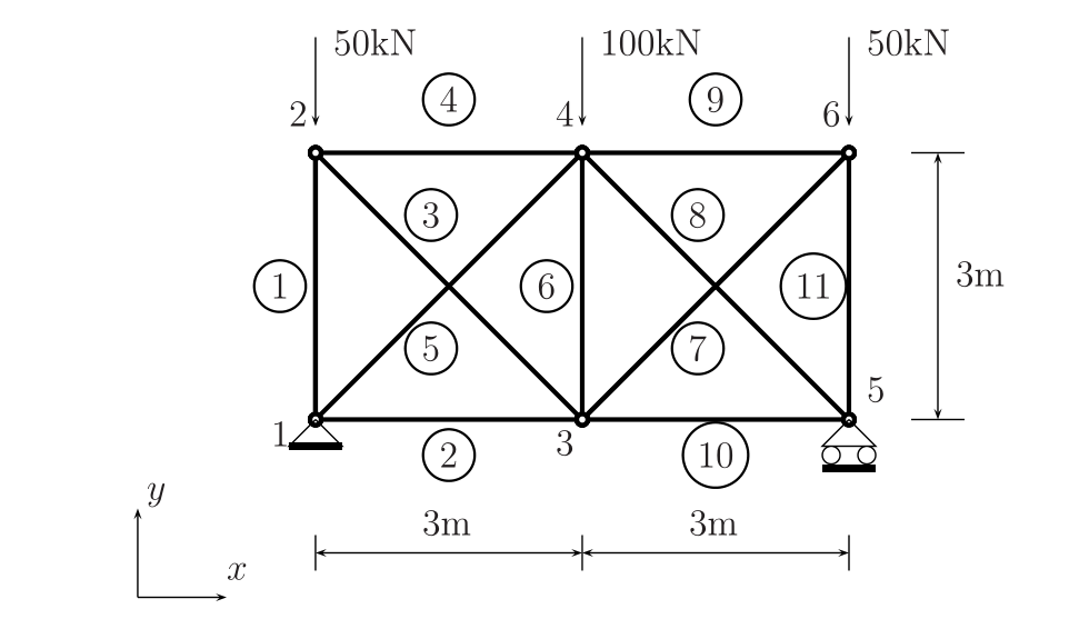
模型参数:
- 杨氏模量E = 70 GPa,泊松比 \(\mu\) = 0.3
- 桁架横截面积 A = \(3e^{-4} m^2\)
- L = 3 m
Abaqus 结果
待补充...
matlab 计算
基于problem4.m 代码,作如下修改即可:
% define model parameters

% unit:SI(m)

p.E = 70e9;

p.A = 3e-4;

p.L = 3;

p.P = 1000*[-50;-100;-50];

disp('单位制:SI(m)')

% define elems and nodes

p.nodes=[0 0 ;  % node's coordinates (x,y)

        0 p.L ;

        p.L 0 ;

        p.L p.L ;

        2*p.L 0 ;

        2*p.L p.L];

p.elems=[1 2 ;

        1 3;

        2 3;

        2 4;

        1 4;

        3 4;

        3 6;

        4 5;

        4 6;

        3 5;

        5 6];

......

% define boundary conditions

% fixed dof

p.fix_dof=[1 2 10]';

% load dof and amplitude

p.load_dof=[4 8 12]';

......
单位制:SI(m)

displacements of dofs :

    1.0000         0

    2.0000         0

    3.0000    0.0071

    4.0000   -0.0090

    5.0000    0.0052

    6.0000   -0.0163

    7.0000    0.0052

    8.0000   -0.0201

    9.0000    0.0105

   10.0000         0

   11.0000    0.0034

   12.0000   -0.0090

forces of dofs :

   1.0e+05 *

    0.0000    0.0000

    0.0000    1.0000

    0.0000    0.0000

    0.0000   -0.5000

    0.0001   -0.0000

    0.0001   -0.0000

    0.0001   -0.0000

    0.0001   -1.0000

    0.0001    0.0000

    0.0001    1.0000

    0.0001         0

    0.0001   -0.5000
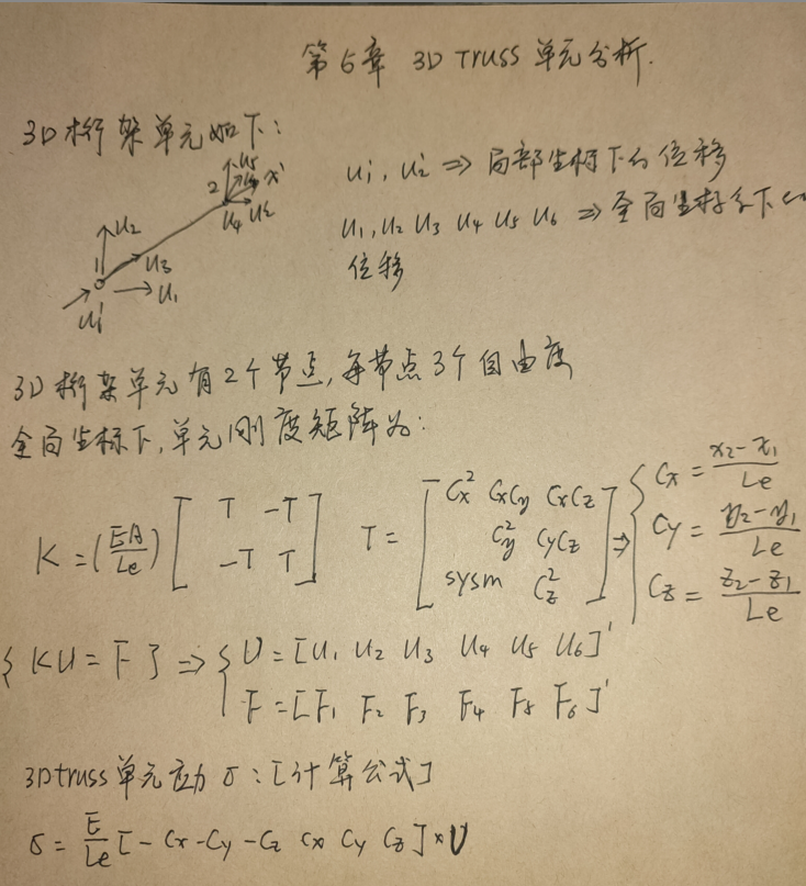
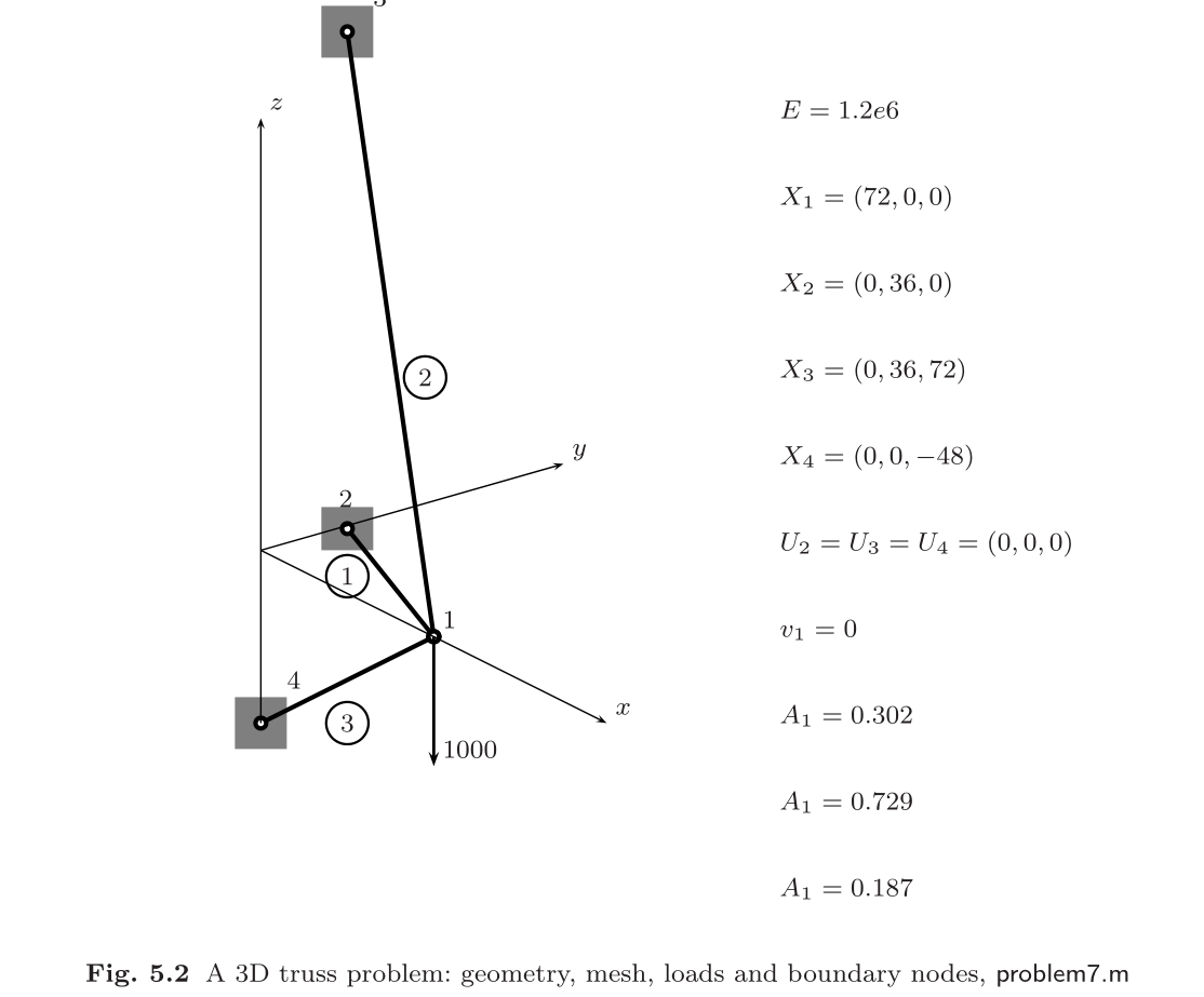
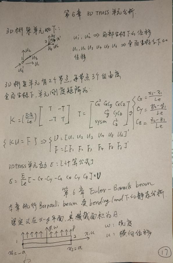
第五章 3D 桁架分析
笔记 - 3d truss 单元刚度矩阵
例题 1
matlab 计算
- problem7.m 代码
% ! problem7.m --> based on <<MATLAB codes for Finite Element Analysis>>
clear ;
clc
format default
p=struct();
% define model parameters
% unit:SI(m)
p.E = 1.2e6;
p.A = [0.302 0.729 0.187]';
p.P = -1000;
disp('单位制:SI(m)')
% define elems and nodes
p.nodes=[72 0 0 ; % node's coordinates (x,y,z)
0 36 0;
0 36 72;
0 0 -48];
p.elems=[1 2 ;
1 3;
1 4];
p.node_num=size(p.nodes,1);
p.elem_num=size(p.elems,1);
p.node_Coord_x=p.nodes(:,1);
p.node_Coord_y=p.nodes(:,2);
p.node_Coord_z=p.nodes(:,3);
% define problem's dimension : 1D/2D/3D;
% = each node's dof
p.problem_dimension=size(p.nodes,2);
% global degree of freedom number
p.global_dof_num=p.problem_dimension*p.node_num;
% define global Nodal displacement colum vector
p.displacements=zeros(p.global_dof_num,1);
p.node_forces=zeros(p.global_dof_num,1);
% define boundary conditions
% fixed dof
p.fix_dof=[2 4 5 6 7 8 9 10 11 12]';
% load dof and amplitude
p.load_dof=3;
% initial global stiffness matrix
p.global_stiffness_matrix=zeros(p.global_dof_num);
% compute all ElemStiffnessMatrix and assembly stiff matrix
elem_global_dof_num=p.problem_dimension*size(p.elems,2);
p.elemStiffs=zeros(elem_global_dof_num,elem_global_dof_num,p.elem_num);
for i=1:p.elem_num
connectivity=p.elems(i,:);
% elem's all dof : a 3d truss node has 2 node,each node have 3 dof,
% i-th node --> U_(3*i-2) / U_(3*i-1) / U_(3*i) dof(displacement of node)
elem_dof=[connectivity(1)*3-2 connectivity(1)*3-1 connectivity(1)*3 ...
connectivity(2)*3-2 connectivity(2)*3-1 connectivity(2)*3];
node1_x=p.node_Coord_x(connectivity(1));
node1_y=p.node_Coord_y(connectivity(1));
node1_z=p.node_Coord_z(connectivity(1));
node2_x=p.node_Coord_x(connectivity(2));
node2_y=p.node_Coord_y(connectivity(2));
node2_z=p.node_Coord_z(connectivity(2));
elem_length=sqrt((node1_x-node2_x).^2+(node1_y-node2_y).^2+(node1_z-node2_z).^2);
Cx=(node2_x-node1_x)/elem_length;
Cy=(node2_y-node1_y)/elem_length;
Cz=(node2_z-node1_z)/elem_length;
T=[Cx*Cx Cx*Cy Cx*Cz;
Cx*Cy Cy*Cy Cy*Cz;
Cx*Cz Cy*Cz Cz*Cz];
k_e=(p.E*p.A(i)/elem_length)*[T -T;-T T];
p.elemStiffs(:,:,i)=k_e;
% assemble stiffness matrix
p.global_stiffness_matrix(elem_dof,elem_dof)=...
p.global_stiffness_matrix(elem_dof,elem_dof)+k_e;
end
% apply boundary condition
p.displacements(p.fix_dof)=0;
p.node_forces(p.load_dof)=p.P;
% solution KU=F
p = solutionStruct(p);
% calculate stress
p.stress=zeros(p.elem_num,1);
for i=1:p.elem_num
connectivity=p.elems(i,:);
% elem's all dof : a 3d truss node has 2 node,each node have 3 dof,
% i-th node --> U_(3*i-2) / U_(3*i-1) / U_(3*i) dof(displacement of node)
elem_dof=[connectivity(1)*3-2 connectivity(1)*3-1 connectivity(1)*3 ...
connectivity(2)*3-2 connectivity(2)*3-1 connectivity(2)*3];
node1_x=p.node_Coord_x(connectivity(1));
node1_y=p.node_Coord_y(connectivity(1));
node1_z=p.node_Coord_z(connectivity(1));
node2_x=p.node_Coord_x(connectivity(2));
node2_y=p.node_Coord_y(connectivity(2));
node2_z=p.node_Coord_z(connectivity(2));
elem_length=sqrt((node1_x-node2_x).^2+(node1_y-node2_y).^2+(node1_z-node2_z).^2);
Cx=(node2_x-node1_x)/elem_length;
Cy=(node2_y-node1_y)/elem_length;
Cz=(node2_z-node1_z)/elem_length;
p.stress(i)=(p.E/elem_length)*[-Cx -Cy -Cz Cx Cy Cz]*p.displacements(elem_dof);
end
% show compute result
disp('displacements of dofs :')
disp([(1:p.global_dof_num)', p.displacements])
disp('forces of dofs :')
disp([(1:p.global_dof_num)',p.node_forces])
disp('3d truss elem stress :')
disp([(1:p.elem_num)',p.stress])
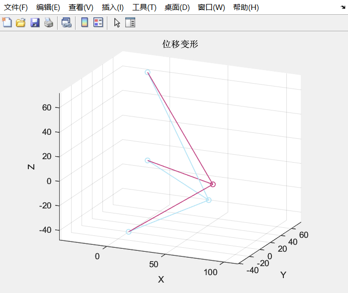
figure
axis equal
% plot undeformed mesh
draw_3Dtruss_mesh(p.nodes,p)
% plot deformed mesh
deformed_node_coordinate=cal_deformed_nodes(p,50.0);
draw_3Dtruss_mesh(deformed_node_coordinate,p)
title('位移变形')
grid on
function draw_3Dtruss_mesh(nodes,p)
xy=zeros(size(p.elems,2)*p.elem_num,p.problem_dimension);
cur1=1;
cur2=0;
for i =1:p.elem_num
connectivity=p.elems(i,:);
attach_node_num=size(connectivity,2);
cur1=cur2+1;
cur2=cur2+attach_node_num;
coord=zeros(attach_node_num,p.problem_dimension);
for j=1:size(connectivity,2)
coord(j,:)=nodes(connectivity(j),:);
end
xy(cur1:cur2,:)=coord;
end
line(xy(:,1),xy(:,2),xy(:,3),"Marker","o","LineWidth",1,"Color",rand(1,3))
end
- 计算结果
单位制:SI(m)

displacements of dofs :

    1.0000   -0.0711

    2.0000         0

    3.0000   -0.2662

    4.0000         0

    5.0000         0

    6.0000         0

    7.0000         0

    8.0000         0

    9.0000         0

   10.0000         0

   11.0000         0

   12.0000         0

forces of dofs :

   1.0e+03 *

    0.0010         0

    0.0020   -0.2232

    0.0030   -1.0000

    0.0040    0.2561

    0.0050   -0.1281

    0.0060         0

    0.0070   -0.7024

    0.0080    0.3512

    0.0090    0.7024

    0.0100    0.4463

    0.0110         0

    0.0120    0.2976

3d truss elem stress :

   1.0e+03 *

    0.0010   -0.9482

    0.0020    1.4454

    0.0030   -2.8685
例题2
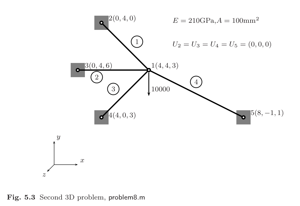
模型参数:
- E = 210000 Mpa,\(\mu\)=0.3
- A = 100 mm^2
- P =-10000 N
Abaqus 结果
waiting...
Matlab 计算
- problem8.m
基于problem7.m,修改参数,即可.
% define model parameters

% unit:SI(mm)

p.E = 210000;

p.A = 100;

p.P = -10000;

disp('单位制:SI(mm)')

% define elems and nodes

p.nodes=[4 4 3 ;  % node's coordinates (x,y,z)

        0 4 0;

        0 4 6;

        4 0 3;

        8 -1 1];

p.elems=[1 2 ;

        1 3;

        1 4;

        1 5];

......

% define boundary conditions

% fixed dof

p.fix_dof=[4:15]';

% load dof and amplitude

p.load_dof=2;

......
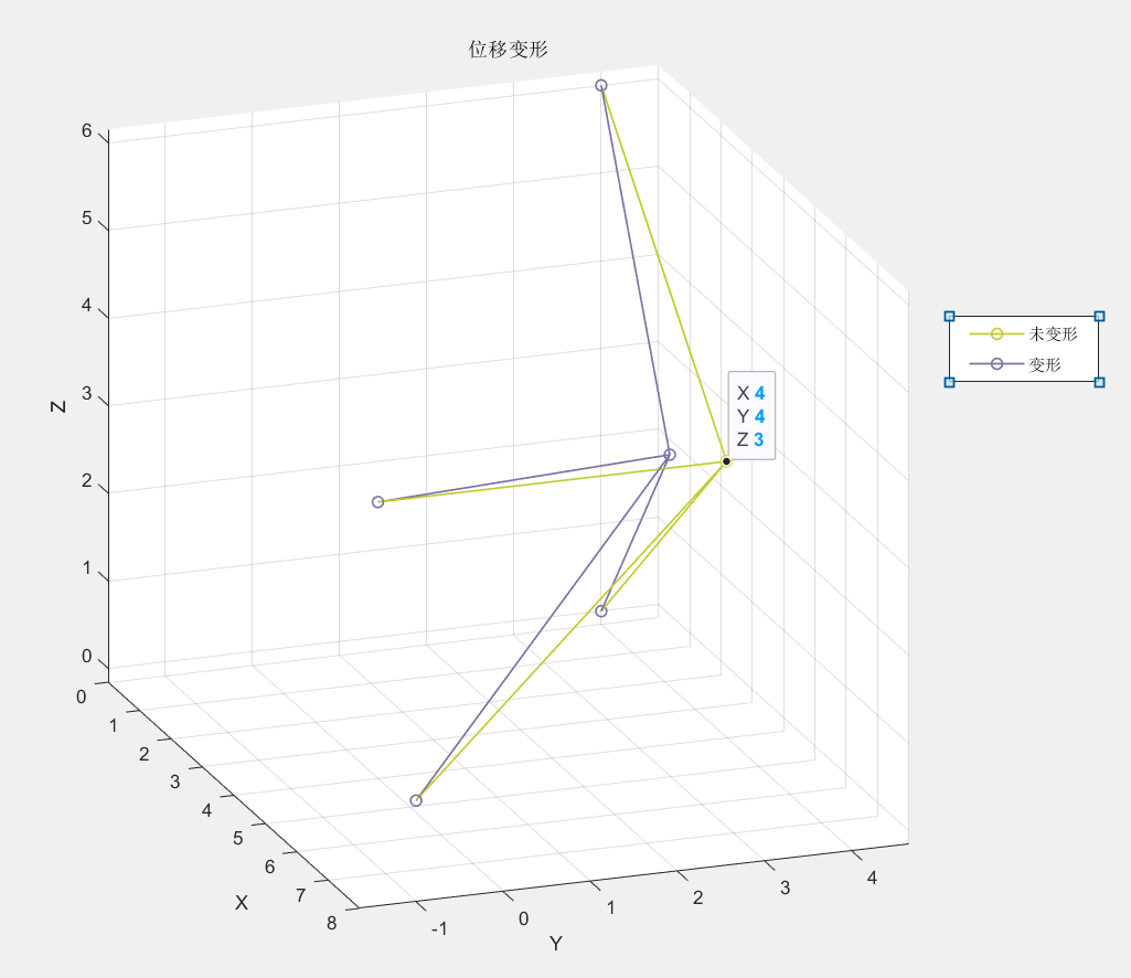
- 计算结果
单位制:SI(mm)

displacements of dofs :

    1.0000   -0.0003

    2.0000   -0.0015

    3.0000    0.0003

forces of dofs :

   1.0e+04 *

    0.0004    0.0271

    0.0005         0

    0.0006    0.0203

    0.0007    0.1355

    0.0008         0

    0.0009   -0.1016

    0.0010         0

    0.0011    0.7968

    0.0012         0

    0.0013   -0.1626

    0.0014    0.2032

    0.0015    0.0813

3d truss elem stress :

    1.0000   -3.3865

    2.0000  -16.9326

    3.0000  -79.6809

    4.0000  -27.2610

deformed nodes:

    3.8791    3.3929    3.1075

         0    4.0000         0

         0    4.0000    6.0000

    4.0000         0    3.0000

    8.0000   -1.0000    1.0000
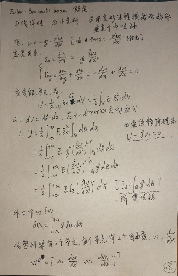
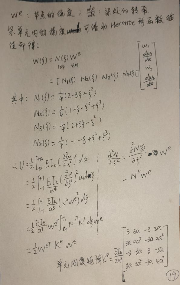
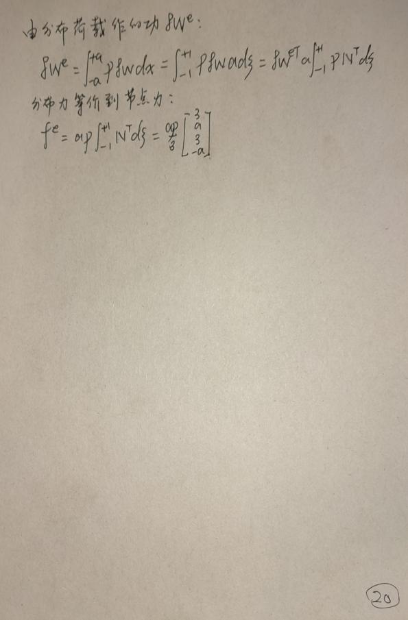
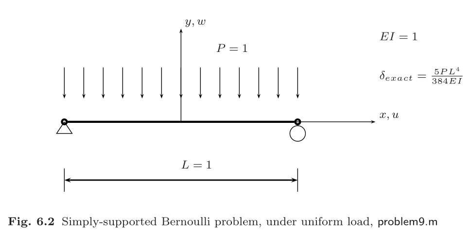
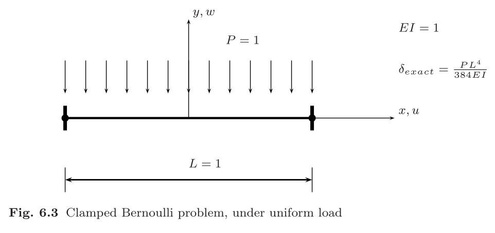
第六章 2D 欧拉-伯努利梁分析
单元刚度矩阵推导
例题 1
consider a simply-supported and clamped Bernoulli beam in bending, under uniform load
Abaqus 计算
Matlab 计算
% ! problem9.m --> based on <<MATLAB codes for Finite Element Analysis>>

clear ;

clc

format default

p=struct();

Case=1;

% define model parameters

% unit:SI(mm)

p.EI = 1;

p.L = 1;

% * distribute force

p.P = -1;

% define elems num of bornoulli beam

p.elem_num=80;

% define problem's dimension : 1D/2D/3D;

%        = each node's dof

p.problem_dimension=2;

% ? -------------------------------

% node's coordinates (x)

p.nodes=linspace(0,p.L,p.elem_num+1)';

p.elems=zeros(p.elem_num,2);

for i=1:p.elem_num

    p.elems(i,1)=i;

    p.elems(i,2)=i+1;

end

p.node_num=size(p.nodes,1);

p.node_Coord_x=p.nodes(:,1);

% global degree of freedom number

p.global_dof_num=2*p.node_num;

% define global Nodal displacement  colum vector

p.displacements=zeros(p.global_dof_num,1);

p.node_forces=zeros(p.global_dof_num,1);

% define boundary conditions

if Case==1

    % Case 01: clamped at x=0

    % fixed dof

    p.fix_dof=[1 2]';

end

if Case==2

    % Case 02: clamped-clamped

    % fixed dof

    p.fix_dof=[1 p.elem_num*2+1 2 p.elem_num*2+2]';

end

if Case==3

    % Case 03: simply supported-simply supported

    p.fix_dof=[1 2*p.elem_num+1]';

end

% initial global stiffness matrix

p.global_stiffness_matrix=zeros(p.global_dof_num);

% compute all ElemStiffnessMatrix and assembly stiff matrix

elem_global_dof_num=p.problem_dimension*size(p.elems,2);

p.elemStiffs=zeros(elem_global_dof_num,elem_global_dof_num,p.elem_num);

for i=1:p.elem_num

    connectivity=p.elems(i,:);

    % elem's all dof : a 3d truss node has 2 node,each node have 2 dof,

    % i-th node --> w_(2*i-1) / dw_(2*i-2) /  dof(displacement of node)

    elem_dof=[connectivity(1)*2-1 connectivity(1)*2  ...

        connectivity(2)*2-1 connectivity(2)*2 ];

    node1_x=p.node_Coord_x(connectivity(1));

    node2_x=p.node_Coord_x(connectivity(2));

    elem_length=node2_x-node1_x;

    a=0.5*elem_length;

    k_e=(p.EI/(a^3))*0.5*[3 3*a -3 3*a;

                        3*a 4*a*a -3*a 2*a*a;

                        -3 -3*a 3 -3*a;

                        3*a 2*a*a -3*a 4*a*a];

    p.elemStiffs(:,:,i)=k_e;

    p.node_forces(elem_dof)=p.node_forces(elem_dof)+((p.P*a/3)*[3 a 3 -a])';

    % assemble stiffness matrix

    p.global_stiffness_matrix(elem_dof,elem_dof)=...

        p.global_stiffness_matrix(elem_dof,elem_dof)+k_e;

end

% apply boundary condition

p.displacements(p.fix_dof)=0;

% solution KU=F

p = solutionStruct_bornoulli_beam(p);

plot(p.node_Coord_x,p.displacements(1:2:2*p.node_num),'.')

minDispalce=min(p.displacements(1:2:2*p.node_num));

text(0.35,0.5*minDispalce,"挠度最小值:"+minDispalce)

if Case==1

    title("Case 01: clamped at x=0")

end

if Case==2

    title("Case 02: clamped-clamped")

end

if Case==3

    title("Case 03: simply supported-simply supported")

end

function new_p=solutionStruct_bornoulli_beam(p)

    % free dof in structure

    free_dof=setdiff((1:p.global_dof_num)',p.fix_dof);

    % solute the equation :KU=F --> U=K\F

    U=p.global_stiffness_matrix(free_dof,free_dof)\p.node_forces(free_dof);

    p.displacements(free_dof)=U;

    % displacements=zeros(p.global_dof_num,1);

    p.node_forces_fu=p.global_stiffness_matrix*p.displacements;

    new_p=p;

end
例题2
matlab 计算
- problem10.m
% ! problem10.m --> based on <<MATLAB codes for Finite Element Analysis>>

clear;

clc;

format compact;

p=struct();

% define model paraeters

p.E=1000000;

p.L=10;

t=p.L/1000;

p.Iz=(1*t^3)/12;

p.P=-1000;

% define elems of bornoulli beam

p.elem_num=20;

% dof of each nornoulli beam nodes

p.bornoulli_node_dof_num=2;

p.spring_k=100;

% -------------------------------

% node's coordinate

p.nodes=linspace(0,p.L,p.elem_num+1)';

p.elems=zeros(p.elem_num,2);

for i=1:p.elem_num

    p.elems(i,1)=i;

    p.elems(i,2)=i+1;

end

p.node_num=size(p.nodes,1);

p.node_Coord_x=p.nodes(:,1);

% global degree of freedom number:

%   ! bornoulli_beam node's dof + 1 spring node's dof

p.global_dof_num=2*p.node_num;

% define global Nodal displacement  colum vector

p.displacements=zeros(p.global_dof_num+1,1);

p.node_forces=zeros(p.global_dof_num+1,1);

% define boundary conditions

%   ! BC: clamped at x=0

p.fix_dof=[1,2,p.global_dof_num+1]';

% initial global stiffness matrix

p.global_stiffness_matrix=zeros(p.global_dof_num+1);

% compute all ElemStiffnessMatrix and assembly stiff matrix

beam_dof_num=p.bornoulli_node_dof_num*size(p.elems,2);

p.elemStiffs=zeros(beam_dof_num,beam_dof_num,p.elem_num);

for i=1:p.elem_num

    connectivity=p.elems(i,:);

    % elem's all dof : a 3d truss node has 2 node,each node have 2 dof,

    % i-th node --> w_(2*i-1) / dw_(2*i-2) /  dof(displacement of node)

    elem_dof=[connectivity(1)*2-1 connectivity(1)*2  ...

        connectivity(2)*2-1 connectivity(2)*2 ];

    node1_x=p.node_Coord_x(connectivity(1));

    node2_x=p.node_Coord_x(connectivity(2));

    elem_length=node2_x-node1_x;

    a=0.5*elem_length;

    k_e=(p.E*p.Iz/(a^3))*0.5*[3 3*a -3 3*a;

                        3*a 4*a*a -3*a 2*a*a;

                        -3 -3*a 3 -3*a;

                        3*a 2*a*a -3*a 4*a*a];

    p.elemStiffs(:,:,i)=k_e;

    p.node_forces(elem_dof)=p.node_forces(elem_dof)+((p.P*a/3)*[3 a 3 -a])';

    % assemble stiffness matrix

    p.global_stiffness_matrix(elem_dof,elem_dof)=...

        p.global_stiffness_matrix(elem_dof,elem_dof)+k_e;

end

% add spring nodes into global_stiffness_matrix

p.global_stiffness_matrix([p.global_dof_num-1,p.global_dof_num+1],[p.global_dof_num-1,p.global_dof_num+1])=...

    p.global_stiffness_matrix([p.global_dof_num-1,p.global_dof_num+1],[p.global_dof_num-1,p.global_dof_num+1])+p.spring_k*[1,-1;-1,1];

% apply boundary condition

p.node_forces(p.fix_dof)=0;

% solution KU=F

p=solutionStruct(p);

% ! display result

disp('Bornoulli beam result !')

disp('beam挠度:')

omega_index=(1:2:p.global_dof_num)';

disp([omega_index,p.displacements(omega_index)])

disp('beam转角:')

theta_index=(2:2:p.global_dof_num)';

disp([theta_index,p.displacements(theta_index)])

disp('beam支反力:')

disp([p.fix_dof,p.node_forces(p.fix_dof)])

plot(p.node_Coord_x,p.displacements(omega_index),'-')

title('Problem10.m')
- 计算结果
Bornoulli beam result !

beam挠度:

   1.0e+05 *

    0.0000         0

    0.0000   -0.1722

    0.0001   -0.6300

    0.0001   -1.2909

    0.0001   -2.0800

    0.0001   -2.9297

    0.0001   -3.7800

    0.0001   -4.5785

    0.0002   -5.2801

    0.0002   -5.8473

    0.0002   -6.2501

    0.0002   -6.4661

    0.0003   -6.4802

    0.0003   -6.2849

    0.0003   -5.8802

    0.0003   -5.2737

    0.0003   -4.4803

    0.0003   -3.5225

    0.0004   -2.4303

    0.0004   -1.2413

    0.0004   -0.0004

beam转角:

   1.0e+05 *

    0.0000         0

    0.0000   -0.6588

    0.0001   -1.1450

    0.0001   -1.4738

    0.0001   -1.6600

    0.0001   -1.7188

    0.0001   -1.6650

    0.0002   -1.5138

    0.0002   -1.2800

    0.0002   -0.9788

    0.0002   -0.6250

    0.0002   -0.2338

    0.0003    0.1800

    0.0003    0.6012

    0.0003    1.0149

    0.0003    1.4062

    0.0003    1.7599

    0.0004    2.0612

    0.0004    2.2949

    0.0004    2.4462

    0.0004    2.4999

beam支反力:

   1.0e+04 *

    0.0001    0.6000

    0.0002    1.2479

    0.0043    0.3750

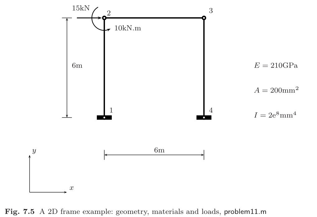
第7章 2d Frame单元静态分析
单元刚度矩阵推导
参见博文:【刚度矩阵推导】2d frame 单元
例题
Matlab 代码
% ! problem10.m --> based on <<MATLAB codes for Finite Element Analysis>>
% ! chpater 7 using 2d-frame element
clear ;
clc
format default
p=struct();
% define model parameters
p.E = 210000; % SI(mm)
p.A = 200;
p.P = [15000 10e6]';
p.Iz=2e8;
% define elems and nodes
p.nodes=[0 0 ; % node's coordinates (x,y)
0 6000 ;
6000 6000 ;
6000 0;];
p.elems=[1 2; 2 3; 3 4;];
p.node_num=size(p.nodes,1);
p.elem_num=size(p.elems,1);
p.node_Coord_x=p.nodes(:,1);
p.node_Coord_y=p.nodes(:,2);
% define problem's dimension = each node's dof
p.problem_dimension=3;
% global degree of freedom number
p.global_dof_num=3*p.node_num;
% define global Nodal displacement colum vector
p.displacements=zeros(p.global_dof_num,1);
p.node_forces=zeros(p.global_dof_num,1);
% define boundary conditions
% fixed dof
p.fix_dof=[1 2 3 10 11 12]';
% load dof and amplitude
p.load_dof=[4 6]';
% initial global stiffness matrix
p.global_stiffness_matrix=zeros(p.global_dof_num);
% compute all ElemStiffnessMatrix and assembly stiff matrix
elem_global_dof_num=p.problem_dimension*size(p.elems,2);
p.elemStiffs=zeros(elem_global_dof_num,elem_global_dof_num,p.elem_num);
for i=1:p.elem_num
connectivity=p.elems(i,:);
% elem's all dof : a 2d frame elem has 2 node,each node have 3 dof,
% i-th node --> U_(3*i-2) and U_(3*i-1) and U_(3*i) dof(displacement of node)
elem_dof=[connectivity(1)*3-2 connectivity(1)*3-1 connectivity(1)*3 connectivity(2)*3-2 connectivity(2)*3-1 connectivity(2)*3];
node1_x=p.node_Coord_x(connectivity(1));
node1_y=p.node_Coord_y(connectivity(1));
node2_x=p.node_Coord_x(connectivity(2));
node2_y=p.node_Coord_y(connectivity(2));
elem_length=sqrt((node1_x-node2_x).^2+(node1_y-node2_y).^2);
l=(node2_x-node1_x)/elem_length;
m=(node2_y-node1_y)/elem_length;
% coordinate transform matrix: U_l=L*U_g
L=[l m 0 0 0 0;
-m l 0 0 0 0;
0 0 1 0 0 0;
0 0 0 l m 0;
0 0 0 -m l 0;
0 0 0 0 0 1;];
% in local coordinates, the stiffness matrix of the frame element is obtained by com-
% bination of the stiffness of the bar element and the Bernoulli beam element
E=p.E;
A=p.A;
Iz=p.Iz;
k_e_local=zeros(elem_global_dof_num,elem_global_dof_num);
k_e_local(1,1)=(E*A)/elem_length;
k_e_local(4,4)=(E*A)/elem_length;
k_e_local(1,4)=-(E*A)/elem_length;
k_e_local(4,1)=-(E*A)/elem_length;
k_e_local(2,2)=12*E*Iz/(elem_length^3);
k_e_local(2,3)=6*E*Iz/(elem_length^2);
k_e_local(2,5)=12*E*Iz/(elem_length^3);
k_e_local(2,6)=6*E*Iz/(elem_length^2);
k_e_local(3,2)=6*E*Iz/(elem_length^2);
k_e_local(5,2)=12*E*Iz/(elem_length^3);
k_e_local(6,2)=6*E*Iz/(elem_length^2);
k_e_local(3,3)=4*E*Iz/(elem_length);
k_e_local(3,5)=-6*E*Iz/(elem_length*elem_length);
k_e_local(3,6)=2*E*Iz/elem_length;
k_e_local(6,3)=2*E*Iz/elem_length;
k_e_local(5,3)=-6*E*Iz/(elem_length*elem_length);
k_e_local(5,5)=12*E*Iz/(elem_length*elem_length*elem_length);
k_e_local(5,6)=-6*E*Iz/(elem_length*elem_length);
k_e_local(6,5)=-6*E*Iz/(elem_length*elem_length);
k_e_local(6,6)=4*E*Iz/elem_length;
k_e_global=L' *k_e_local *L;
p.elemStiffs(:,:,i)=k_e_global;
% assemble stiffness matrix
p.global_stiffness_matrix(elem_dof,elem_dof)=...
p.global_stiffness_matrix(elem_dof,elem_dof)+k_e_global;
end
% apply boundary condition
p.displacements(p.fix_dof)=0;
p.node_forces(p.load_dof)=p.P;
% solution KU=F
p = solutionStruct(p);
% show compute result
disp('displacements of dofs :')
disp([(1:p.global_dof_num)', p.displacements])
disp('forces of dofs :')
disp([(1:p.global_dof_num)',p.node_forces])
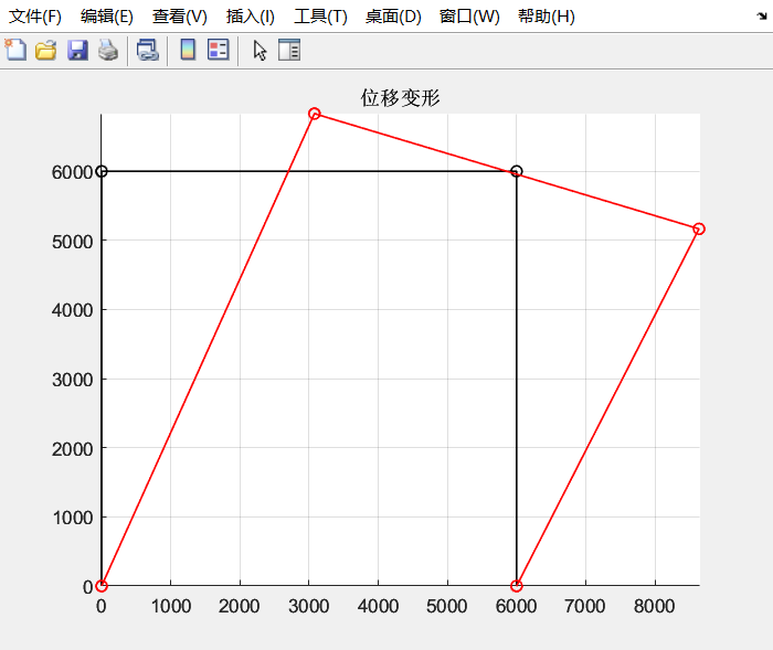
figure
axis equal
% plot undeformed mesh
draw_2Dtruss_mesh(p.nodes,p,'black')
deform_scale=500;
deformed_node_coordinate=[p.node_Coord_x+deform_scale*p.displacements(3*(1:p.node_num)-2), ...
p.node_Coord_y+deform_scale*p.displacements(3*(1:p.node_num)-1)];
% plot deformed mesh
draw_2Dtruss_mesh(deformed_node_coordinate,p,'red')
title('位移变形')
grid on
第八章 3d Frame单元静态分析
略
第九章 analysis of grids
略
第十章 Timoshenko beams 静态分析
与欧拉-伯努利梁公式不同,Timoshenko梁公式考虑了横向剪切变形.因此,它能够模拟较薄或较厚的梁.本章对Timoshenko梁的静力弯曲、自由振动和屈曲进行了分析.
10.Timoshenko梁的静力分析-Formulation
有限元方法[Matlab]-笔记的更多相关文章
- 常微分方程初值问题:单步方法 [MATLAB]
#先上代码后补笔记# #可以直接复制粘贴调用的MATLAB函数代码!# 1. 朗格-库塔(Runge-Kutta)方法族 目前只实现了四阶Runge-Kutta方法. function [ YMat ...
- 数值积分:基于牛顿-柯茨公式的定步长和自适应积分方法 [MATLAB]
#先上代码后补笔记# #可以直接复制粘贴使用的MATLAB函数!# 1. 定步长牛顿-柯茨积分公式 function [ integration ] = CompoInt( func, left, r ...
- Android Studio调试方法学习笔记
(注:本人所用Android Studio的Keymap已设为Eclipse copy) 1.设置断点 只有设置断点,才好定位要调试什么地方,否则找不到要调试的地方,无法调试.(调试过程中也可以增加断 ...
- angular模块和组件之间传递信息和操作流程的方法(笔记)
angular的模块之间,以及controller.directive等组件之间,是相对独立的,用以实现解耦合. 为实现相互之间传递信息及操作流程,有以下一些机制: 1.事件机制: $scope.$b ...
- JS数组中every(),filter(),forEach(),map(),some()方法学习笔记!
ES5中定义了五种数组的迭代方法:every(),filter(),forEach(),map(),some(). 每个方法都接受两个参数:要在每一项运行的函数(必选)和运行该函数的作用域的对象-影响 ...
- dojo/dom-construct.toDom方法学习笔记
toDom方法用来将html标签字符串转化成DOM节点.1.7之后toDom方法被分配到了dom-construct模块. require(["dojo/dom-construct" ...
- 产品需求文档(PRD)的写作方法之笔记一
1.写前准备(思维导图): http://www.woshipm.com/?p=80070 1.在写之前,请先很区分清楚什么是MRD文档(市场需求文档),BRD文档(商业需求文档),什么是PRD文档( ...
- java static 方法使用笔记
有入参的static方法,可以正常使用 static的作用是申明:这是类的静态方法,什么时候都可以调用,可以传入入参,也可以不传. 上代码: 1.带静态方法的类: public class MakeP ...
- juquery验证插件validation addMethod方法使用笔记
该方法有三个api接口参数,name,method,messages addMethod(name,method,message)方法 参数 name 是添加的方法的名字. 参数 method 是一个 ...
- zepto.1.1.6.js源码中的each方法学习笔记
each方法接受要遍历的对象和对应的回调函数作为参数,它的作用是: 1.如果要遍历的对象是类似数组的形式(以该对象的length属性值的类型是否为number类型来判断),那么就把以要遍历的对象为执行 ...
随机推荐
- 【前端】HTML编码效提升:快速生成HTML标签
目录 1.生成多级标签 2.生成同级标签 3.生成注释 4.生成多个相同标签 5.生成带class标签 6生成带id标签. 7.生成带内容标签1 8.生成带内容标签2 9.生成带属性标签 GIF演示: ...
- dockercompose配置ulimit
在 Docker Compose 文件中设置 ulimit 的方法如下: 在 Docker Compose 文件的 services 块中,为您要设置 ulimit 的服务添加 ulimits 子块, ...
- redis中是没有Long类型的
redis中没有Long类型,存储进去后取出来会是Interger类型.需要自行转化,不可直接强转.否则将CCE. 本人在处理springboot的redisTemplate封装时发生了这个异常.解决 ...
- 使用Spring提供的BeanUtils.copyProperties()方法报错:Could not copy property 'xxx' from source to target
使用Spring提供的BeanUtils.copyProperties()方法报错:Could not copy property 'xxx' from source to target; neste ...
- 性能优化!突破性能瓶颈的尖兵CPU Cache
大家好,我是呼噜噜,今天我们来介绍计算机的储存器之一,CPU高速缓冲存储器也叫高速缓存,CPU Cache 缓存这个专业术语,在计算机世界中是经常使用到的.它并不是CPU所独有的,比如cdn缓存网站信 ...
- Qt数据库应用19-图片转pdf
一.前言 用户的需求真的是千奇百怪,刚做完不同页面横向纵向排版的需求,又来个需要图片转pdf的需求,提供静态函数直接使用. 经过这么些年的社会的毒打,我的原则是:用户是上帝和大爷,尽量站在用户的角度换 ...
- Qt编写地图综合应用28-闪烁点图
一.前言 Qt除了内置了各种UI组件以外,还直接集成了浏览器控件,注意哦这可是跨平台的浏览器控件哦,在5.6版本以前集成的是webkit,以后集成的是webengine,使得程序的灵活性拓展性大大增强 ...
- Python中导入模块的import命令的语法
- 基于Netty,徒手撸IM(一):IM系统设计篇
本文收作者"大白菜"分享,有改动.注意:本系列是给IM初学者的文章,IM老油条们还望海涵,勿喷! 1.引言 这又是一篇基于Netty的IM编码实践文章,因为合成一篇内容太长,读起来 ...
- C Primer Plus 第6版 第二章 编程练习参考答案
编译环境VS Code+WSL GCC /*第一题*************************/ #include<stdio.h> int main() { printf(&quo ...