Deep learning with Python 学习笔记（3）

本节介绍基于Keras的使用预训练模型方法

想要将深度学习应用于小型图像数据集，一种常用且非常高效的方法是使用预训练网络。预训练网络(pretrained network)是一个保存好的网络，之前已在大型数据集(通常是大规模图像分类任务)上训练好

使用预训练网络有两种方法:特征提取(feature extraction)和微调模型(fine-tuning)

特征提取是使用之前网络学到的表示来从新样本中提取出有趣的特征。然后将这些特征输入一个新的分类器，从头开始训练 ，简言之就是用提取的特征取代原始输入图像来直接训练分类器

图像分类的卷积神经网络包含两部分:首先是一系列池化层和卷积层，最后是一个密集连接分类器。第一部分叫作模型的卷积基(convolutional base)。对于卷积神经网络而言，特征提取就是取出之前训练好的网络的卷积基，在上面运行新数据，然后在输出上面训练一个新的分类器

重复使用卷积基的原因在于卷积基学到的表示可能更加通用，因此更适合重复使用

某个卷积层提取的表示的通用性(以及可复用性)取决于该层在模型中的深度。模型中更靠近底部的层提取的是局部的、高度通用的特征图(比如视觉边缘、颜色和纹理)，而更靠近顶部的层提取的是更加抽象的概念(比如“猫耳朵”或“狗眼睛”)。所以如果你的新数据集与原始模型训练的数据集有很大差异，那么最好只使用模型的前几层来做特征提取，而不是使用整个卷积基

可以从 keras.applications 模块中导入一些内置的模型如

• Xception
• Inception V3
• ResNet50
• VGG16
• VGG19
• MobileNet

实例化VGG16卷积基

from keras.applications import VGG16
conv_base = VGG16(weights='imagenet', include_top=False, input_shape=(150, 150, 3))

weights 指定模型初始化的权重检查点，include_top 指定模型最后是否包含密集连接分类器，input_shape 是输入到网络中的图像张量的形状

可以使用conv_base.summary()来查看网络结构

可见网络最后一层的输出特征图形状为 (4, 4, 512)，此时我们需要在该特征上添加一个密集连接分类器，有两种方法可以选择

1. 在你的数据集上运行卷积基，将输出保存成硬盘中的 Numpy 数组，然后用这个数据作为输入，输入到独立的密集连接分类器中

这种方法速度快，计算代价低，因为对于每个输入图像只需运行一次卷积基，而卷积基是目前流程中计算代价最高的。但出于同样的原因，这种方法不允许你使用数据增强

1. 在顶部添加 Dense 层来扩展已有模型（即 conv_base），并在输入数据上端到端地运行整个模型

这样你可以使用数据增强，因为每个输入图像进入模型时都会经过卷积基。但出于同样的原因，这种方法的计算代价比第一种要高很多

以下将使用在 ImageNet 上训练的 VGG16 网络的卷积基从猫狗图像中提取有趣的特征，然后在这些特征上训练一个猫狗分类器

第一种方法，保存你的数据在 conv_base 中的输出，然后将这些输出作为输入用于新模型

不使用数据增强的快速特征提取

import os
import numpy as np
from keras.preprocessing.image import ImageDataGenerator
from keras.applications import VGG16
from keras import models
from keras import layers
from keras import optimizers
import matplotlib.pyplot as plt

conv_base = VGG16(weights='imagenet', include_top=False, input_shape=(150, 150, 3))
base_dir = 'C:\\Users\\fan\\Desktop\\testDogVSCat'
train_dir = os.path.join(base_dir, 'train')
validation_dir = os.path.join(base_dir, 'validation')
test_dir = os.path.join(base_dir, 'test')
datagen = ImageDataGenerator(rescale=1./255)
batch_size = 20

# 图像及其标签提取为 Numpy 数组
def extract_features(directory, sample_count):
    features = np.zeros(shape=(sample_count, 4, 4, 512))
    labels = np.zeros(shape=(sample_count))
    generator = datagen.flow_from_directory(directory, target_size=(150, 150), batch_size=batch_size, class_mode='binary')
    i = 0
    for inputs_batch, labels_batch in generator:
        features_batch = conv_base.predict(inputs_batch)
        features[i * batch_size: (i + 1) * batch_size] = features_batch
        labels[i * batch_size: (i + 1) * batch_size] = labels_batch
        i += 1
        if i * batch_size >= sample_count:
            break
    return features, labels

train_features, train_labels = extract_features(train_dir, 2000)
validation_features, validation_labels = extract_features(validation_dir, 1000)
test_features, test_labels = extract_features(test_dir, 1000)
# 将(samples, 4, 4, 512)展平为(samples, 8192)
train_features = np.reshape(train_features, (2000, 4 * 4 * 512))
validation_features = np.reshape(validation_features, (1000, 4 * 4 * 512))
test_features = np.reshape(test_features, (1000, 4 * 4 * 512))

model = models.Sequential()
model.add(layers.Dense(256, activation='relu', input_dim=4 * 4 * 512))
model.add(layers.Dropout(0.5))
model.add(layers.Dense(1, activation='sigmoid'))

model.compile(optimizer=optimizers.RMSprop(lr=2e-5),
              loss='binary_crossentropy', metrics=['acc'])
history = model.fit(train_features, train_labels, epochs=30,
                    batch_size=20, validation_data=(validation_features, validation_labels))

acc = history.history['acc']
val_acc = history.history['val_acc']
loss = history.history['loss']
val_loss = history.history['val_loss']
epochs = range(1, len(acc) + 1)
plt.plot(epochs, acc, 'bo', label='Training acc')
plt.plot(epochs, val_acc, 'b', label='Validation acc')
plt.title('Training and validation accuracy')
plt.legend()
plt.figure()
plt.plot(epochs, loss, 'bo', label='Training loss')
plt.plot(epochs, val_loss, 'b', label='Validation loss')
plt.title('Training and validation loss')
plt.legend()
plt.show()

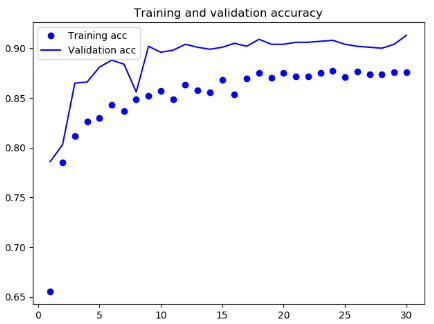
结果

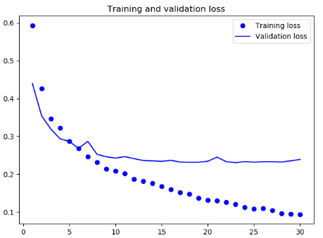
可见，在训练集上的表现要比之前好很多，不过还是出现了一定程度的过拟合

第二种方法

使用数据增强的特征提取

注：扩展 conv_base 模型，然后在输入数据上端到端地运行模型

因为我们要使用的卷积基不需要重新训练，所以我们需要将卷积基冻结

在 Keras 中，冻结网络的方法是将其 trainable 属性设为 False

 conv_base.trainable = False

使用len(model.trainable_weights)可以查看可以训练的权重张量个数，此时应该注意每一层有两个张量(主权重矩阵和偏置向量)

Demo如下

import os
from keras.preprocessing.image import ImageDataGenerator
from keras.applications import VGG16
from keras import models
from keras import layers
from keras import optimizers
import matplotlib.pyplot as plt

conv_base = VGG16(weights='imagenet', include_top=False, input_shape=(150, 150, 3))
base_dir = 'C:\\Users\\fan\\Desktop\\testDogVSCat'
train_dir = os.path.join(base_dir, 'train')
validation_dir = os.path.join(base_dir, 'validation')
test_dir = os.path.join(base_dir, 'test')
datagen = ImageDataGenerator(rescale=1./255)
test_datagen = ImageDataGenerator(rescale=1./255)
batch_size = 20

train_datagen = ImageDataGenerator(rescale=1./255, rotation_range=40, width_shift_range=0.2,
                                   height_shift_range=0.2, shear_range=0.2, zoom_range=0.2,
                                   horizontal_flip=True, fill_mode='nearest')
train_generator = train_datagen.flow_from_directory(train_dir,  target_size=(150, 150),  batch_size=batch_size, class_mode='binary')
validation_generator = test_datagen.flow_from_directory(validation_dir, target_size=(150, 150), batch_size=batch_size, class_mode='binary')

conv_base.trainable = False
model = models.Sequential()
model.add(conv_base)
model.add(layers.Flatten())
model.add(layers.Dense(256, activation='relu'))
model.add(layers.Dense(1, activation='sigmoid'))

model.compile(loss='binary_crossentropy', optimizer=optimizers.RMSprop(lr=2e-5), metrics=['acc'])
history = model.fit_generator(train_generator, steps_per_epoch=100, epochs=30, validation_data=validation_generator, validation_steps=50)

acc = history.history['acc']
val_acc = history.history['val_acc']
loss = history.history['loss']
val_loss = history.history['val_loss']
epochs = range(1, len(acc) + 1)
plt.plot(epochs, acc, 'bo', label='Training acc')
plt.plot(epochs, val_acc, 'b', label='Validation acc')
plt.title('Training and validation accuracy')
plt.legend()
plt.figure()
plt.plot(epochs, loss, 'bo', label='Training loss')
plt.plot(epochs, val_loss, 'b', label='Validation loss')
plt.title('Training and validation loss')
plt.legend()
plt.show()

结果

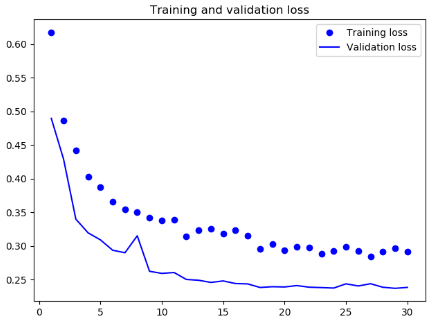
可见，此时没有出现明显的过拟合现象，在验证集上出现了更好的结果

此处应该可以使用数据增强的方式扩充我们的数据集，然后再通过第一种方法来训练分类器

模型微调

另一种广泛使用的模型复用方法是模型微调（fine-tuning），与特征提取互为补充。微调是指将其顶部的几层“解冻”，并将这解冻的几层和新增加的部分联合训练，此处的顶层指的是靠近分类器的一端

此时我们只是微调顶层的原因是

卷积基中更靠底部的层编码的是更加通用的可复用特征，而更靠顶部的层编码的是更专业化的特征。微调这些更专业化的特征更加有用，因为它们需要在你的新问题上改变用途

训练的参数越多，过拟合的风险越大

微调网络的步骤如下

1. 在已经训练好的基网络（base network）上添加自定义网络
2. 冻结基网络
3. 训练所添加的部分
4. 解冻基网络的一些层
5. 联合训练解冻的这些层和添加的部分

冻结直到某一层的方法

conv_base.trainable = True
set_trainable = False
for layer in conv_base.layers:
	if layer.name == 'block5_conv1':
 		set_trainable = True
 		if set_trainable:
 		layer.trainable = True
 	else:
 		layer.trainable = False

微调网络时可以使用学习率非常小的 RMSProp 优化器来实现，太大的权重更新可能会对我们的网络造成很大的破坏

为了让图像更具可读性，可以将每个损失和精度都替换为指数移动平均值，从而让曲线变得平滑

def smooth_curve(points, factor=0.8):
 smoothed_points = []
 for point in points:
 	if smoothed_points:
 		previous = smoothed_points[-1]
 		smoothed_points.append(previous * factor + point * (1 - factor))
 	else:
 		smoothed_points.append(point)
 return smoothed_points

精度的是损失值的分布，而不是平均值

Deep learning with Python 学习笔记（4）

Deep learning with Python 学习笔记（2）