信号处理——Hilbert端点效应浅析

作者：桂。

时间：2017-03-05  19:29:12

链接：http://www.cnblogs.com/xingshansi/p/6506405.html

声明：转载请注明出处，谢谢。

---

前言

本文为Hilbert变换分析的补充，主要介绍Hilbert变换中的端点效应，内容拟分两部分展开：

　　1）Gibbs现象介绍；

　　2）端点效应分析；

内容为自己一家之言，其中不合理的地方，希望各位告诉我，反正改不改是我的事(●'◡'●)

一、Gibbs现象

关于Gibbs的理论推导，可以参考郑君里的《信号与系统》上册（第二版，P97~101），里边有详细的理论分析。也可参考：维基百科，里边有一张图很形象：

给出对应的代码（用该程序，借助MATLAB便可以生成.gif图）：

%% 代码介绍========================================================================
%% Title:
%  1) Fourier series approximation of square wave.
%  2) Demonstration of Gibbs phenomenon (verification of Fig. 3.9 of [1])
%% Author:
%  Ankit A. Bhurane (ankit.bhurane@gmail.com)
%% Expression:
% The Fourier series approximation of a square wave signal existing between
% -Tau/2 to Tau/2 and period of T0 will have the form:
%
% Original signal to be approximated:
%                         :
%               __________:__________  A
%              |          :          |
%              |          :          |
%              |          :          |
%    __________|          :          |__________
% -T0/2     -Tau/2        0        Tau/2       T0/2
%                         :
%                         :
%
% Its Fourier series approximation:
%
%                  Inf
%                  ___
%         A*Tau   \     / sin(pi*n*Tau/T0)                    \
% r(t) = -------   |   | ------------------ exp^(j*n*2*pi/T0*t) |
%          T0     /___  \  (pi*n*Tau/T0)                      /
%               n = -Inf
%
% The left term inside summation are the Fourier series coeffs (Cn). The
% right term is the Fourier series kernel.
% Tau: range of square wave, T: period of the square wave,
% t: time variable, n: number of retained coefficients.
%
%% Observations:
% 1) As number of retained coefficients tends to infinity, the approximated
% signal value at the discontinuity converge to half the sum of values on
% either side.
% 2) Ripples does not decrease with increasing coefficients with
% approximately 9% overshoot.
% 3) Energy in the error between original and approximated signal, reduces
% as the number of retained coefficients are increased.
%
%% References:
% [1] Oppenheim, Willsky, Nawab, "Signals and Systems", PHI, Second edition
% [2] Dean K. Frederick and A. Bruce Carlson, "Fourier series" section in
%     Linear systems in communication and control
%% Last Modified: Sept 24, 2013.
%% Copyright (c) 2013-2014 | Ankit A. Bhurane
%%

　　

clc; clear all; close all;

% Specification
A = 1; % Peak-to-peak amplitude of square wave
Tau = 10; % Total range in which the square wave is defined (here -5 to 5)
T0 = 20; % Period (time of repeatation of square wave), here 10
C = 200; % Coefficients (sinusoids) to retain
N = 1001; % Number of points to consider
t = linspace(-(T0-Tau),(T0-Tau),N); % Time axis
X = zeros(1,N); X(t>=-Tau/2 & t<=Tau/2) = A; % Original signal
R = 0; % Initialize the approximated signal
k = -C:C; % Fourier coefficient number axis
f = zeros(1,2*C+1); % Fourier coefficient values

% Loop for plotting approximated signals for different retained coeffs.
for c = 0:C % Number of retained coefficients
    for n = -c:c % Summation range (See equation above in comments)

        % Sinc part of the Fourier coefficients calculated separately
        if n~=0
            Sinc = (sin(pi*n*Tau/T0)/((pi*n*Tau/T0))); % At n NOTEQUAL to 0
        else
            Sinc = 1; % At n EQUAL to 0
        end
        Cn = (A*Tau/T0)*Sinc; % Actual Fourier series coefficients
        f(k==n) = Cn; % Put the Fourier coefficients at respective places
        R = R + Cn*exp(1j*n*2*pi/T0.*t); % Sum all the coefficients
    end

    R = real(R); % So as to get rid of 0.000000000i (imaginary) factor
    Max = max(R); Min = min(R); M = max(abs(Max),abs(Min)); % Maximum error
    Overshoot = ((M-A)/A)*100; % Overshoot calculation
    E = sum((X-R).^2); % Error energy calculation

    % Plots:
    % Plot the Fourier coefficients
    subplot 211; stem(k,f,'m','LineWidth',1); axis tight; grid on;
    xlabel('Fourier coefficient index');ylabel('Magnitude');
    title('Fourier coefficients');

    % Plot the approximated signal
    subplot 212; plot(t,X,t,R,'m','LineWidth',1); axis tight; grid on;
    xlabel('Time (t)'); ylabel('Amplitude');
    title(['Approximation for N = ', num2str(c),...
    '. Overshoot = ',num2str(Overshoot),'%','. Error energy: ',num2str(E)])

    pause(0.1); % Pause for a while
    R = 0; % Reset the approximation to calculate new one
end

　　简而言之：

• 对于跳变的点，傅里叶变换的分量只能是能量收敛，而不是一致（幅度）收敛；
• 对于跳变的点，如门函数/方波，信号由低频到高频众多分量组合而成。

故对于连续时域信号，Fourier级数只能无限项逼近，不能完全一致。

二、端点效应

　　A-理论解释

借用之前博文的一张图：

连续信号到离散信号需要进行采样，由于有无穷多项，采样率对于高频的部分（因为无穷多项）难以满足Nyquist采样定理，因此会出现失真，这也就是端点效应的理论解释。失真的根本原因在时域采样，频域采样步骤只不过影响频域分辨率，即所谓的栅栏效应，但不是造成失真的根本原因。

　　B-现象分析

为了验证理论，此处采样一个正弦信号进行分析，按连续信号来看其Hilbert变换应该是余弦信号。

给出代码：

clc;clear all;close all;
fs = 2000;
f0 = 80;
t = 0:1/fs:.1;
sig = sin(2*pi*f0*t);
sig_ref = -cos(2*pi*f0*t);
sig_hilbert = hilbert(sig);
figure;
subplot 311
plot(t,sig,'k','linewidth',2);hold on;
plot(t,sig_ref,'r.-','linewidth',2);hold on;
plot(t,imag(sig_hilbert),'b','linewidth',2);hold on;
legend('原信号','余弦信号','Hilbert变换信号','localization','best');
ylim([-2,2]);
grid on;
%频谱
f = linspace(0,fs,length(t));
subplot 312
plot(f,abs(fft(sig)),'k');hold on;
plot(f,abs(fft(sig_hilbert)),'r');hold on;
legend('原信号','Hilbert变换信号','localization','best');
grid on;

　　对应的结果图：

时域：

可以看到明显的端点效应（说是端点效应，如果间断点在中间位置，一样会有该效应，毕竟都是Nyquist定理下的误差嘛）。

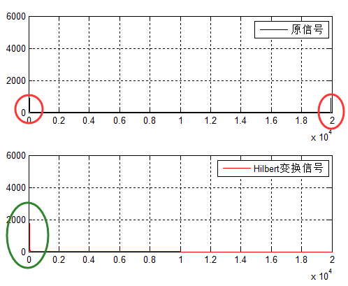
频域：

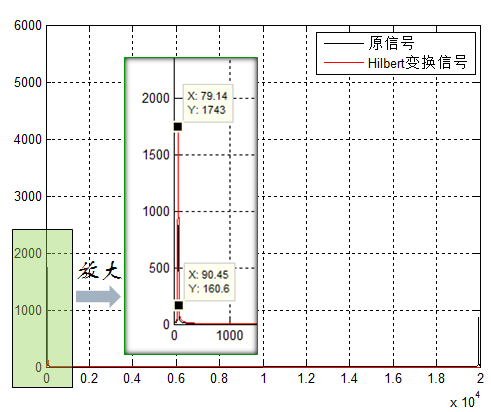
采样率取得够大了，理论上正弦信号Hilbert之后应该是一个单边的冲击。但频谱显示，峰值旁边的一个点，幅度达到160.6，这也印证了能量的泄露。

发现端点效应，与前文理论对应：Hilbert就是一个频域的变相器，本质也是fourier变换，是不是也因为跳变点（即信号中的Gibbs问题）？观察频谱，峰值旁边的点，幅值有160.5大小，我们计算原信号

2*sig(1)-sig(2)

　　得到结果是：-0.4820，而对于没有的点，应该是默认是0的，因此端点算是一个跳变点了。

注意：端点效应是相对于连续信号来讲，存在失真，从而出现误差。对于数字信号，Hilbert变换结果就是该正弦数字信号的精确表达，即逆Hilbert可以完全恢复出正弦信号。给一张Hilbert变换后，进行逆Hilbert变换的code及示意图：

clc;clear all;close all;
fs = 2000;
f0 = 40;
t = 0:1/fs:.1;
sig = sin(2*pi*f0*t);
sig_hilbert = -imag(hilbert(imag(hilbert(sig))));
figure;
plot(t,sig,'k','linewidth',2);hold on;
plot(t,sig_hilbert,'r--','linewidth',2);
ylim([-2,2]);
grid on;

　　从图中，可以看到从Hilbert结果恢复的信号与原信号完全一致！这也印证了上文的观点：失真在时域采样，而不在频域采样。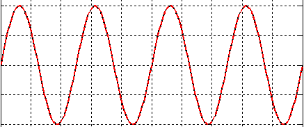

下面再做一组实验，验证推断：
思路——只要保证2sig(1)-sig(2)逼近0，理论上是不是就没有边界效应了？
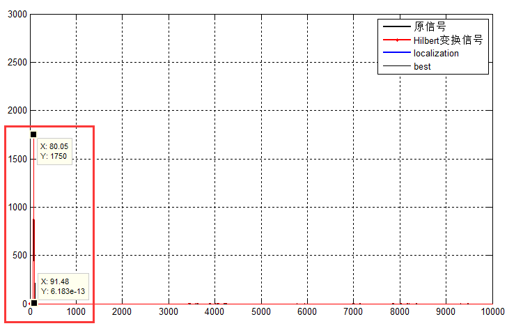
此时：2*sig(1)-sig(2)=1.5873e-05，再来看看结果图：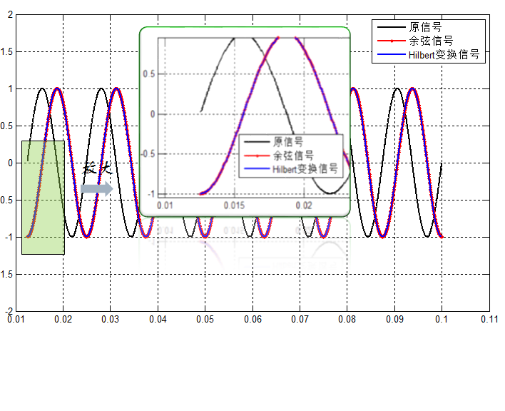

再来看看频谱，没错，峰值旁边的点压的很小（6.183e-13），符合预期。

此处代码：

clc;clear all;close all;
fs = 20000;
f0 = 80;
t = 0.01255:1/fs:.1;%t = 0.0252:1/fs:.1则没有跳变。
sig = sin(2*pi*f0*t);
2*sig(1)-sig(2)
sig_ref = -cos(2*pi*f0*t);
sig_hilbert = hilbert(sig);
figure;
subplot 211
plot(t,sig,'k','linewidth',2);hold on;
plot(t,sig_ref,'r.-','linewidth',2);hold on;
plot(t,imag(sig_hilbert),'b','linewidth',2);hold on;
legend('原信号','余弦信号','Hilbert变换信号','localization','best');
ylim([-2,2]);
grid on;
%频谱
f = linspace(0,fs,length(t));
subplot 212
plot(f,abs(fft(sig)),'k');hold on;
plot(f,abs(fft(sig_hilbert)),'r');hold on;
legend('原信号','Hilbert变换信号','localization','best');
ylim([0 6000]);
grid on;

基于这个基本要点，很多方法对信号：预测、延拓、镜像等操作，以消除或者降低端点效应。为什么用2*sig(1)-sig(2)呢，这是因为实验的函数为sin，在0附近sinx~x ，严格意义上应该是2*f(1)-f(2)≈ 0 。f是函数表达式，而且实际中信号不是单一频点，仅仅通过两个点判断也是不够的。
只是消除端点方法不同，但端点现象的本质一致。
多说一句：Hilbert将双边谱压成单边，这让频域滤波等操作方便了不少。

参考：

Gibbs phenomen:https://en.wikipedia.org/wiki/Gibbs_phenomenon