机器学习作业（三）多类别分类与神经网络——Python(numpy)实现

题目太长了！下载地址【传送门】

第1题

简述：识别图片上的数字。

 import numpy as np
 import scipy.io as scio
 import matplotlib.pyplot as plt
 import scipy.optimize as op

 #显示图片数据
 def displayData(X):
     m = np.size(X, 0)  #X的行数，即样本数量
     n = np.size(X, 1)  #X的列数，即单个样本大小
     example_width = int(np.round(np.sqrt(n)))  #单张图片宽度
     example_height = int(np.floor(n / example_width))  #单张图片高度
     display_rows = int(np.floor(np.sqrt(m)))  #显示图中，一行多少张图
     display_cols = int(np.ceil(m / display_rows))  #显示图中，一列多少张图片
     pad = 1  #图片间的间隔
     display_array = - np.ones((pad + display_rows * (example_height + pad),
                             pad + display_cols * (example_width + pad)))  #初始化图片矩阵
     curr_ex = 0  #当前的图片计数
     #将每张小图插入图片数组中
     for j in range(0, display_rows):
         for i in range(0, display_cols):
             if curr_ex >= m:
                 break
             max_val = np.max(abs(X[curr_ex, :]))
             jstart = pad + j * (example_height + pad)
             istart = pad + i * (example_width + pad)
             display_array[jstart: (jstart + example_height), istart: (istart + example_width)] = \
                 np.array(X[curr_ex, :]).reshape(example_height, example_width) / max_val
             curr_ex = curr_ex + 1
         if curr_ex >= m:
             break
     display_array = display_array.T
     plt.imshow(display_array,cmap=plt.cm.gray)
     plt.axis('off')
     plt.show()

 #计算hθ(z)
 def sigmoid(z):
     g = 1.0 / (1.0 + np.exp(-z))
     return g

 #计算cost
 def lrCostFunction(theta, X, y, lamb):
     theta = np.array(theta).reshape((np.size(theta), 1))
     m = np.size(y)
     h = sigmoid(np.dot(X, theta))
     J = 1 / m * (-np.dot(y.T, np.log(h)) - np.dot((1 - y.T), np.log(1 - h)))
     theta2 = theta[1:, 0]
     Jadd = lamb / (2 * m) * np.sum(theta2 ** 2)
     J = J + Jadd
     return J.flatten()

 #计算梯度
 def gradient(theta, X, y, lamb):
     theta = np.array(theta).reshape((np.size(theta), 1))
     m = np.size(y)
     h = sigmoid(np.dot(X, theta))
     grad = 1/m*np.dot(X.T, h - y)
     theta[0,0] = 0
     gradadd = lamb/m*theta
     grad = grad + gradadd
     return grad.flatten()

 #θ计算
 def oneVsAll(X, y, num_labels, lamb):
     m = np.size(X, 0)
     n = np.size(X, 1)
     all_theta = np.zeros((num_labels, n+1))
     one = np.ones(m)
     X = np.insert(X, 0, values=one, axis=1)
     for c in range(0, num_labels):
         initial_theta = np.zeros(n+1)
         y_t = (y==c)
         result = op.minimize(fun=lrCostFunction, x0=initial_theta, args=(X, y_t, lamb), method='TNC', jac=gradient)
         all_theta[c, :] = result.x
     return all_theta

 #计算准确率
 def predictOneVsAll(all_theta, X):
     m = np.size(X, 0)
     num_labels = np.size(all_theta, 0)
     p = np.zeros((m, 1))  #用来保存每行的最大值
     g = np.zeros((np.size(X, 0), num_labels))  #用来保存每次分类后的结果（一共分类了10次，每次保存到一列上）
     one = np.ones(m)
     X = np.insert(X, 0, values=one, axis=1)
     for c in range(0, num_labels):
         theta = all_theta[c, :]
         g[:, c] = sigmoid(np.dot(X, theta.T))
     p = g.argmax(axis=1)
     # print(p)
     return p.flatten()

 #加载数据文件
 data = scio.loadmat('ex3data1.mat')
 X = data['X']
 y = data['y']
 y = y%10  #因为数据集是考虑了matlab从1开始，把0的结果保存为了10，这里进行取余，将10变回0
 m = np.size(X, 0)
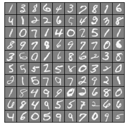
 rand_indices = np.random.randint(0,m,100)
 sel = X[rand_indices, :]
 displayData(sel)

 #计算θ
 lamb = 0.1
 num_labels = 10
 all_theta = oneVsAll(X, y, num_labels, lamb)
 # print(all_theta)

 #计算预测的准确性
 pred = predictOneVsAll(all_theta, X)
 # np.set_printoptions(threshold=np.inf)
 #在计算这个上遇到了一个坑：
 #pred输出的是[[...]]的形式，需要flatten变成1维向量，y同样用flatten变成1维向量
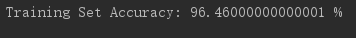
 acc = np.mean(pred == y.flatten())*100
 print('Training Set Accuracy:',acc,'%')

运行结果：

第2题

简介：使用神经网络实现数字识别（Θ已提供）

 import numpy as np
 import scipy.io as scio
 import matplotlib.pyplot as plt
 import scipy.optimize as op

 #显示图片数据
 def displayData(X):
     m = np.size(X, 0)  #X的行数，即样本数量
     n = np.size(X, 1)  #X的列数，即单个样本大小
     example_width = int(np.round(np.sqrt(n)))  #单张图片宽度
     example_height = int(np.floor(n / example_width))  #单张图片高度
     display_rows = int(np.floor(np.sqrt(m)))  #显示图中，一行多少张图
     display_cols = int(np.ceil(m / display_rows))  #显示图中，一列多少张图片
     pad = 1  #图片间的间隔
     display_array = - np.ones((pad + display_rows * (example_height + pad),
                             pad + display_cols * (example_width + pad)))  #初始化图片矩阵
     curr_ex = 0  #当前的图片计数
     #将每张小图插入图片数组中
     for j in range(0, display_rows):
         for i in range(0, display_cols):
             if curr_ex >= m:
                 break
             max_val = np.max(abs(X[curr_ex, :]))
             jstart = pad + j * (example_height + pad)
             istart = pad + i * (example_width + pad)
             display_array[jstart: (jstart + example_height), istart: (istart + example_width)] = \
                 np.array(X[curr_ex, :]).reshape(example_height, example_width) / max_val
             curr_ex = curr_ex + 1
         if curr_ex >= m:
             break
     display_array = display_array.T
     plt.imshow(display_array,cmap=plt.cm.gray)
     plt.axis('off')
     plt.show()

 #计算hθ(z)
 def sigmoid(z):
     g = 1.0 / (1.0 + np.exp(-z))
     return g

 #实现神经网络
 def predict(theta1, theta2, X):
     m = np.size(X,0)
     p = np.zeros((np.size(X, 0), 1))
     #第二层计算
     one = np.ones(m)
     X = np.insert(X, 0, values=one, axis=1)
     a2 = sigmoid(np.dot(X, theta1.T))
     #第三层计算
     one = np.ones(np.size(a2,0))
     a2 = np.insert(a2, 0, values=one, axis=1)
     a3 = sigmoid(np.dot(a2, theta2.T))
     p = a3.argmax(axis=1) + 1  #y的值为1-10，所以此处0-9要加1
     return p.flatten()

 #读取数据文件
 data = scio.loadmat('ex3data1.mat')
 X = data['X']
 y = data['y']
 m = np.size(X, 0)
 rand_indices = np.random.randint(0,m,100)
 sel = X[rand_indices, :]
 # displayData(sel)

 theta = scio.loadmat('ex3weights.mat')
 theta1 = theta['Theta1']
 theta2 = theta['Theta2']

 #预测准确率
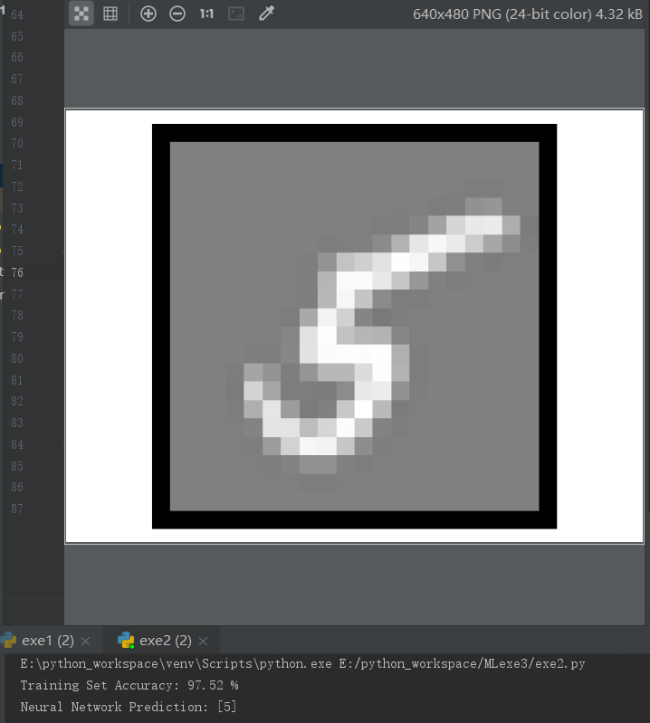
 pred = predict(theta1, theta2, X)
 acc = np.mean(pred == y.flatten())*100
 print('Training Set Accuracy:',acc,'%')

 #识别单张图片
 for i in range(0, m):
     it = np.random.randint(0, m, 1)
     it = it[0]
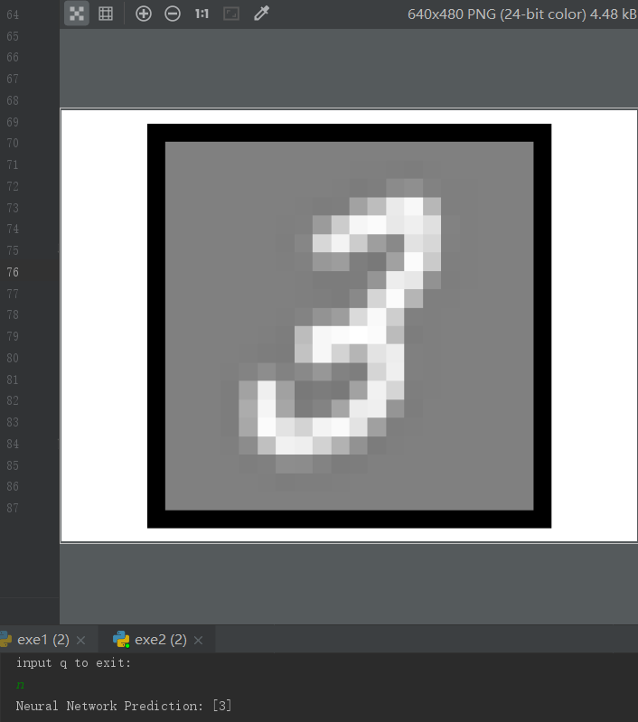
     displayData(X[it:it+1, :])
     pred = predict(theta1, theta2, X[it:it+1, :])
     print('Neural Network Prediction:', pred)
     print('input q to exit:')
     cin = input()
     if cin == 'q':
         break

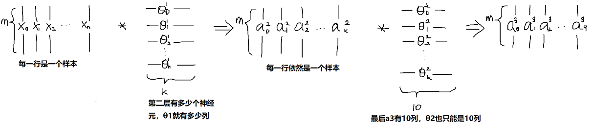
神经网络的矩阵表示分析：

运行结果：