R Tidyverse dplyr包学习笔记2
Tidyverse 学习笔记
1.gapminder 我理解的gapminder应该是一个内置的数据集
加载之后使用
> # Load the gapminder package

> library(gapminder)

> # Load the dplyr package

> library(dplyr)

> # Look at the gapminder dataset

> gapminder

A tibble: 1,704 x 6

   country     continent  year lifeExp      pop gdpPercap

   <fct>       <fct>     <int>   <dbl>    <int>     <dbl>

 1 Afghanistan Asia       1952    28.8  8425333      779.

 2 Afghanistan Asia       1957    30.3  9240934      821.

 3 Afghanistan Asia       1962    32.0 10267083      853.

 4 Afghanistan Asia       1967    34.0 11537966      836.

 5 Afghanistan Asia       1972    36.1 13079460      740.

 6 Afghanistan Asia       1977    38.4 14880372      786.

 7 Afghanistan Asia       1982    39.9 12881816      978.

 8 Afghanistan Asia       1987    40.8 13867957      852.

 9 Afghanistan Asia       1992    41.7 16317921      649.

10 Afghanistan Asia       1997    41.8 22227415      635.

 ... with 1,694 more rows
1.1 filter 函数
解释:过滤/筛选,按条件,可以有很多条件
gapminder %>%filter(year==2002,country=="China")

A tibble: 1 x 6

  country continent  year lifeExp        pop gdpPercap

  <fct>   <fct>     <int>   <dbl>      <int>     <dbl>

1 China   Asia       2002    72.0 1280400000     3119.
1.2 排序函数arrange,默认升序,参数desc降序
> # Sort in ascending order of lifeExp

> gapminder %>%

    arrange(lifeExp)

 A tibble: 1,704 x 6

   country      continent  year lifeExp     pop gdpPercap

   <fct>        <fct>     <int>   <dbl>   <int>     <dbl>

 1 Rwanda       Africa     1992    23.6 7290203      737.

 2 Afghanistan  Asia       1952    28.8 8425333      779.

 3 Gambia       Africa     1952    30    284320      485.

 4 Angola       Africa     1952    30.0 4232095     3521.

 5 Sierra Leone Africa     1952    30.3 2143249      880.

 6 Afghanistan  Asia       1957    30.3 9240934      821.

 7 Cambodia     Asia       1977    31.2 6978607      525.

 8 Mozambique   Africa     1952    31.3 6446316      469.

 9 Sierra Leone Africa     1957    31.6 2295678     1004.

10 Burkina Faso Africa     1952    32.0 4469979      543.

... with 1,694 more rows

按照lifeExp 降序

> # Sort in descending order of lifeExp

> gapminder %>%

    arrange(desc(lifeExp))

 A tibble: 1,704 x 6

   country          continent  year lifeExp       pop gdpPercap

   <fct>            <fct>     <int>   <dbl>     <int>     <dbl>

 1 Japan            Asia       2007    82.6 127467972    31656.

 2 Hong Kong, China Asia       2007    82.2   6980412    39725.

 3 Japan            Asia       2002    82   127065841    28605.

 4 Iceland          Europe     2007    81.8    301931    36181.

 5 Switzerland      Europe     2007    81.7   7554661    37506.

 6 Hong Kong, China Asia       2002    81.5   6762476    30209.

 7 Australia        Oceania    2007    81.2  20434176    34435.

 8 Spain            Europe     2007    80.9  40448191    28821.

 9 Sweden           Europe     2007    80.9   9031088    33860.

10 Israel           Asia       2007    80.7   6426679    25523.

 ... with 1,694 more rows
筛选和排序组合使用:
> library(gapminder)

> library(dplyr)

>

> # Filter for the year 1957, then arrange in descending order of population

> gapminder%>%filter(year==1957)%>%arrange(desc(pop))

A tibble: 142 x 6

   country        continent  year lifeExp       pop gdpPercap

   <fct>          <fct>     <int>   <dbl>     <int>     <dbl>

 1 China          Asia       1957    50.5 637408000      576.

 2 India          Asia       1957    40.2 409000000      590.

 3 United States  Americas   1957    69.5 171984000    14847.

 4 Japan          Asia       1957    65.5  91563009     4318.

 5 Indonesia      Asia       1957    39.9  90124000      859.

 6 Germany        Europe     1957    69.1  71019069    10188.

 7 Brazil         Americas   1957    53.3  65551171     2487.

 8 United Kingdom Europe     1957    70.4  51430000    11283.

 9 Bangladesh     Asia       1957    39.3  51365468      662.

10 Italy          Europe     1957    67.8  49182000     6249.

... with 132 more rows
2 mutute 函数
2.1 修改变量,并且将新变量增加到数据框或者矩阵的左侧
> # Use mutate to change lifeExp to be in months

> gapminder%>%mutate(lifeExp=12*lifeExp)

 A tibble: 1,704 x 6

   country     continent  year lifeExp      pop gdpPercap

   <fct>       <fct>     <int>   <dbl>    <int>     <dbl>

 1 Afghanistan Asia       1952    346.  8425333      779.

 2 Afghanistan Asia       1957    364.  9240934      821.

 3 Afghanistan Asia       1962    384. 10267083      853.

 4 Afghanistan Asia       1967    408. 11537966      836.

 5 Afghanistan Asia       1972    433. 13079460      740.

 6 Afghanistan Asia       1977    461. 14880372      786.

 7 Afghanistan Asia       1982    478. 12881816      978.

 8 Afghanistan Asia       1987    490. 13867957      852.

 9 Afghanistan Asia       1992    500. 16317921      649.

10 Afghanistan Asia       1997    501. 22227415      635.

... with 1,694 more rows

>
2.2 增加新的变量
>  Use mutate to create a new column called lifeExpMonths

> gapminder%>%mutate(lifeExpMonths=12*lifeExp)

 A tibble: 1,704 x 7

   country     continent  year lifeExp      pop gdpPercap lifeExpMonths

   <fct>       <fct>     <int>   <dbl>    <int>     <dbl>         <dbl>

 1 Afghanistan Asia       1952    28.8  8425333      779.          346.

 2 Afghanistan Asia       1957    30.3  9240934      821.          364.

 3 Afghanistan Asia       1962    32.0 10267083      853.          384.

 4 Afghanistan Asia       1967    34.0 11537966      836.          408.

 5 Afghanistan Asia       1972    36.1 13079460      740.          433.

 6 Afghanistan Asia       1977    38.4 14880372      786.          461.

 7 Afghanistan Asia       1982    39.9 12881816      978.          478.

 8 Afghanistan Asia       1987    40.8 13867957      852.          490.

 9 Afghanistan Asia       1992    41.7 16317921      649.          500.

10 Afghanistan Asia       1997    41.8 22227415      635.          501.

... with 1,694 more rows
2.3 combine
> library(gapminder)

> library(dplyr)

> # Filter, mutate, and arrange the gapminder dataset

> gapminder%>%filter(year==2007)%>%mutate(

  lifeExpMonths=12 * lifeExp,

  )%>%arrange(desc(lifeExpMonths))

 A tibble: 142 x 7

   country          continent  year lifeExp       pop gdpPercap lifeExpMonths

   <fct>            <fct>     <int>   <dbl>     <int>     <dbl>         <dbl>

 1 Japan            Asia       2007    82.6 127467972    31656.          991.

 2 Hong Kong, China Asia       2007    82.2   6980412    39725.          986.

 3 Iceland          Europe     2007    81.8    301931    36181.          981.

 4 Switzerland      Europe     2007    81.7   7554661    37506.          980.

 5 Australia        Oceania    2007    81.2  20434176    34435.          975.

 6 Spain            Europe     2007    80.9  40448191    28821.          971.

 7 Sweden           Europe     2007    80.9   9031088    33860.          971.

 8 Israel           Asia       2007    80.7   6426679    25523.          969.

 9 France           Europe     2007    80.7  61083916    30470.          968.

10 Canada           Americas   2007    80.7  33390141    36319.          968.

... with 132 more rows
3 浅谈:ggplot2 绘图
基本的制图,不添加任何图形元素是可以看下面的小demo,但是用到其他的元素了,就可以
https://cran.r-project.org/web/packages/ggplot2/ggplot2.pdf这个说明文当还是挺全面的
library(gapminder)

library(dplyr)

library(ggplot2)

gapminder_1952 <- gapminder %>%

  filter(year == 1952)

Change to put pop on the x-axis and gdpPercap on the y-axis

ggplot(gapminder_1952, aes(x = pop, y = gdpPercap)) +

  geom_point()

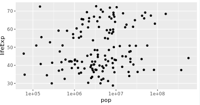
3.1 x坐标取对数
zheyang
> library(gapminder)

> library(dplyr)

> library(ggplot2)

>

> gapminder_1952 <- gapminder %>%

    filter(year == 1952)

>

> # Change this plot to put the x-axis on a log scale

> ggplot(gapminder_1952, aes(x = pop, y = lifeExp)) +

    geom_point()+

    scale_x_log10()
> library(gapminder)

> library(dplyr)

> library(ggplot2)

>

> gapminder_1952 <- gapminder %>%

    filter(year == 1952)

>

> # Change this plot to put the x-axis on a log scale

> ggplot(gapminder_1952, aes(x = pop, y = lifeExp)) +

    geom_point()+

    scale_x_log10()+

    scale_y_log10()
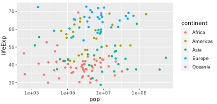
3.2 设置color和size
设置国家的颜色是不一样的

 gapminder_1952 <- gapminder %>%

    filter(year == 1952)

>

> # Scatter plot comparing pop and lifeExp, with color representing continent

> ggplot(gapminder_1952,aes(x=pop,y=lifeExp,colour= continent))+geom_point()+

  scale_x_log10()
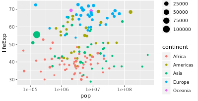
3.3 设置size
> gapminder_1952 <- gapminder %>%

    filter(year == 1952)

>

> # Add the size aesthetic to represent a country's gdpPercap

> ggplot(gapminder_1952, aes(x = pop, y = lifeExp, color = continent,size=gdpPercap)) +

    geom_point() +

    scale_x_log10()
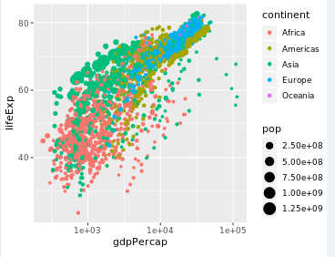
3.4 Faceting
Faceting is a powerful way to understand subsets of your data separately
可以按照条件分类显示数据
facet_wrap(~condi):按照condi来显示数据分类
and size representing population, faceted by year

> ggplot(gapminder,aes(x=gdpPercap,y=lifeExp,colour=continent,size=pop))+

  geom_point()+

  scale_x_log10()

> facet_wrap(~year)

<ggproto object: Class FacetWrap, Facet, gg>

    compute_layout: function

    draw_back: function

    draw_front: function

    draw_labels: function

    draw_panels: function

    finish_data: function

    init_scales: function

    map_data: function

    params: list

    setup_data: function

    setup_params: function

    shrink: TRUE

    train_scales: function

    vars: function

    super:  <ggproto object: Class FacetWrap, Facet, gg>
4.summarize
类似与summary的函数,可以描述性输出。
但是里面的内置函数只有:sum,mean,median,min,max。
 Filter for 1957 then summarize the median life expectancy and the maximum GDP per capita

gapminder%>%filter(year==1957)%>%summarize(

medianLifeExp=median(lifeExp),

maxGdpPercap=max(gdpPercap)

)
5 group_by
分组求解
> # Find median life expectancy and maximum GDP per capita in each continent in 1957

> gapminder%>%filter(year==1957)%>%group_by(continent)%>%summarize(

  medianLifeExp=median(lifeExp),

  maxGdpPercap=max(gdpPercap)

  )

 A tibble: 5 x 3

  continent medianLifeExp maxGdpPercap

  <fct>             <dbl>        <dbl>

1 Africa             40.6        5487.

2 Americas           56.1       14847.

3 Asia               48.3      113523.

4 Europe             67.6       17909.

5 Oceania            70.3       12247.
可以有多个条件进行分组
> # Find median life expectancy and maximum GDP per capita in each continent/year combination

> gapminder%>%group_by(continent,year)%>%summarize(

  medianLifeExp=median(lifeExp),

  maxGdpPercap=max(gdpPercap)

  )

A tibble: 60 x 4

# Groups:   continent [5]

   continent  year medianLifeExp maxGdpPercap

   <fct>     <int>         <dbl>        <dbl>

 1 Africa     1952          38.8        4725.

 2 Africa     1957          40.6        5487.

 3 Africa     1962          42.6        6757.

 4 Africa     1967          44.7       18773.

 5 Africa     1972          47.0       21011.

 6 Africa     1977          49.3       21951.

 7 Africa     1982          50.8       17364.

 8 Africa     1987          51.6       11864.

 9 Africa     1992          52.4       13522.

10 Africa     1997          52.8       14723.

# ... with 50 more rows
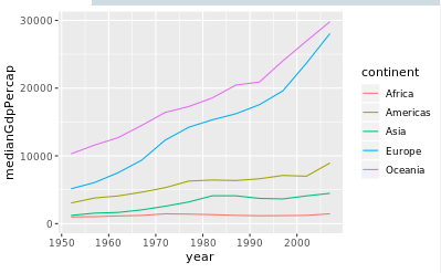
6.expand_limits(y=0)
让y轴从0开始
ibrary(gapminder)

library(dplyr)

library(ggplot2)

# Summarize medianGdpPercap within each continent within each year: by_year_continent

by_year_continent<-gapminder%>%group_by(continent,year)%>%summarize(

medianGdpPercap=median(gdpPercap))

# Plot the change in medianGdpPercap in each continent over time

ggplot(by_year_continent,aes(x=year,y=medianGdpPercap,colour=continent))+geom_point()+

expand_limits(y = 0)
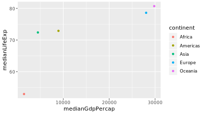
> # Use a scatter plot to compare the median GDP and median life expectancy

> ggplot(by_continent_2007,aes(x=medianLifeExp,y=medianGdpPercap,colour=continent))+geom_point()

> library(gapminder)

> library(dplyr)

> library(ggplot2)

>

> # Summarize the median GDP and median life expectancy per continent in 2007

> by_continent_2007 <- gapminder %>%

    filter(year == 2007) %>%

    group_by(continent) %>%

    summarize(medianGdpPercap = median(gdpPercap),

              medianLifeExp = median(lifeExp))

>

> # Use a scatter plot to compare the median GDP and median life expectancy

> ggplot(by_continent_2007, aes(x = medianGdpPercap, y = medianLifeExp, color = continent)) +

    geom_point()
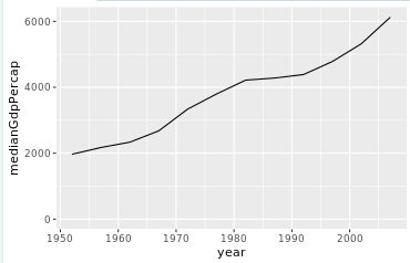
line plot
线图
上面画的都是散点图
library(gapminder)

library(dplyr)

library(ggplot2)

# Summarize the median gdpPercap by year, then save it as by_year

by_year<-gapminder%>%group_by(year)%>%summarize(medianGdpPercap=median(gdpPercap))

# Create a line plot showing the change in medianGdpPercap over time

ggplot(by_year, aes(x = year, y = medianGdpPercap)) +

  geom_line() +

  expand_limits(y = 0)
直线图和散点图的区别就是geom_point()与geom_line()
library(ggplot2)
>
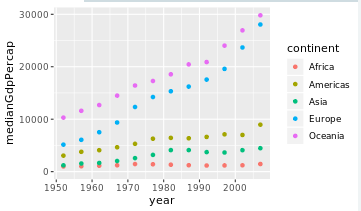
> # Summarize the median gdpPercap by year & continent, save as by_year_continent
> by_year_continent<-gapminder%>%group_by(year,continent)%>%summarize(
medianGdpPercap=median(gdpPercap)
)
>
> # Create a line plot showing the change in medianGdpPercap by continent over time
> ggplot(by_year_continent,aes(x = year, y = medianGdpPercap,color=continent))+
geom_line()+
expand_limits(y = 0)
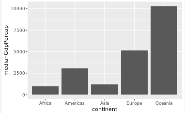
bar plot
 library(gapminder)

> library(dplyr)

> library(ggplot2)

>

> # Summarize the median gdpPercap by year and continent in 1952

> by_continent<-gapminder%>%filter(year==1952)%>%group_by(continent)%>%summarize(

  medianGdpPercap=median(gdpPercap))

>

> # Create a bar plot showing medianGdp by continent

> ggplot(by_continent,aes(x=continent,y=medianGdpPercap))+geom_col()
library(ggplot2)

gapminder_1952 <- gapminder %>%

  filter(year == 1952) %>%

  mutate(pop_by_mil = pop / 1000000)

# Create a histogram of population (pop_by_mil)

ggplot(gapminder_1952,aes(x=pop_by_mil))+

geom_histogram(bins=50)

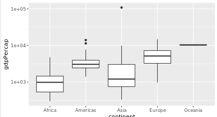
boxplot
# Create a boxplot comparing gdpPercap among continents

> ggplot(gapminder_1952,aes(x=continent,y=gdpPercap))+

  geom_boxplot()+

  scale_y_log10()

> ggplot(gapminder_1952,aes(x=continent,y=gdpPercap))+

  geom_boxplot()+

  scale_y_log10()
ggtitle
如果给表加上标题就用ggtitle("标题名")
gapminder_1952 <- gapminder %>%

    filter(year == 1952)

>

> # Add a title to this graph: "Comparing GDP per capita across continents"

> ggplot(gapminder_1952, aes(x = continent, y = gdpPercap)) +

    geom_boxplot() +

    scale_y_log10()+

    ggtitle("Comparing GDP per capita across continents")
不同的图形按照ggplot来说只是修改geom_*的参数
ggplot2
R Tidyverse dplyr包学习笔记2的更多相关文章
- R语言与机器学习学习笔记
人工神经网络(ANN),简称神经网络,是一种模仿生物神经网络的结构和功能的数学模型或计算模型.神经网络由大量的人工神经元联结进行计算.大多数情况下人工神经网络能在外界信息的基础上改变内部结构,是一种自 ...
- R语言与显著性检验学习笔记
R语言与显著性检验学习笔记 一.何为显著性检验 显著性检验的思想十分的简单,就是认为小概率事件不可能发生.虽然概率论中我们一直强调小概率事件必然发生,但显著性检验还是相信了小概率事件在我做的这一次检验 ...
- R语言函数化学习笔记3
R语言函数化学习笔记3 R语言常用的一些命令函数 1.getwd()查看当前R的工作目录 2.setwd()修改当前工作目录 3.str()可以输出指定对象的结构(类型,位置等),同理还有class( ...
- R语言dplyr包初探
昨天学了一下R语言dplyr包,处理数据框还是很好用的.记录一下免得我忘记了... 先写一篇入门的,以后有空再写一篇详细的用法. #dplyr learning library(dplyr) #fil ...
- R语言函数化学习笔记6
R语言函数化学习笔记 1.apply函数 可以让list或者vector的元素依次执行一遍调用的函数,输出的结果是list格式 2.sapply函数 原理和list一样,但是输出的结果是一个向量的形式 ...
- R parallel包学习笔记2
这个部分我在datacamp上面学习笔记,可视化的性能很差,使用的函数也很少. 可以参考一下大佬的博客园个人感觉他们讲的真的很详细 https://cosx.org/2016/09/r-and-par ...
- R语言函数话学习笔记5
使用Tidyverse完成函数化编程 (参考了家翔学长的笔记) 1.magrittr包的使用 里面有很多的管道函数,,可以减少代码开发时间,提高代码可读性和维护性 1.1 四种pipeline 1.1 ...
- 【数据分析 R语言实战】学习笔记 第八章 方差分析与R实现
方差分析泛应用于商业.经济.医学.农业等诸多领域的数量分析研究中.例如商业广告宣传方面,广告效果可能会受广告式.地区规模.播放时段.播放频率等多个因素的影响,通过方差分析研究众多因素中,哪些是主要的以 ...
- pandas包学习笔记
目录 zip Importing & exporting data Plotting with pandas Visual exploratory data analysis 折线图 散点图 ...
随机推荐
- 调整markdown css样式
H1标题 H2标题 H3标题 H4标题 H5标题 H6标题 段落: 世情薄,人情恶.雨送黄昏花易落.晓风干,泪痕残.欲笺心事,独语斜阑.难,难,难! 人成各,今非昨.病魂常似秋千索.角声寒,夜阑珊.怕 ...
- window10 cmd 常见命令
AT 计划在计算机上运行的命令和程序. ATTRIB 显示或更改文件属性. BREAK 设置或清除扩展式 CTRL+C 检查. CACLS 显示或修改文件的访问控制列表(ACLs). CALL 从另一 ...
- 清北学堂—2020.1提高储备营—Day 4 morning(数论)
qbxt Day 4 morning --2020.1.20 济南 主讲:李奥 目录一览 1.一些符号与基本知识 2.拓展欧几里得,逆元与欧拉定理 3.线性筛法与积性函数(非重点) 总知识点:数论 一 ...
- ggEditor流程图增加网格背景
参考官方文档: https://www.yuque.com/antv/g6/plugin.tool.grid react-ggEditor如何使用 import { Flow } from 'gg-e ...
- nginx 反向代理及 https 证书配置
nginx 反向代理及 https 证书配置 author: yunqimg(ccxtcxx0) 1. 编译安装nginx 从官网下载 nginx源码, 并编译安装. ./configure --pr ...
- matplotlib制作图表数据
import matplotlib.pyplot as plt import matplotlib fig=plt.figure() labels=['陆地','海洋'] data=[29,71] p ...
- 用友UAP NC 开发环境抛出"JDK默认编辑器找不到"
此节点是升级65之前开发的,已经很久不使用,今天在开发环境使用,点查询抛出此异常. 最后问了人解决方法,就是往JRE系统库加入对应的jar包
- 剑指offer-面试题10-斐波那契数列-递归循环
/* 题目:求斐波那契数列的第n项 */ /* 思路: f(n) = 0 n=0, 1 n=1, f(n-1) + f(n-2) n>1 */ int Fibonacci(int n){ if( ...
- P4802 [CCO 2015]路短最
Problem 这题的题意是 求一条 经过 起点和终点的 最长路径.且一个点只能经过一次. 我们设定 \(dis_{i,j}\) 为 i 到 j 的距离(应该没有重边) 要注意的是 不能用 \(Flo ...
- django cookie session 自定义分页
cookie cookie的由来 http协议是无状态的,犹如人生若只如初见,每次都是初次.由此我们需要cookie来保持状态,保持客户端和服务端的数据通信. 什么是cookie Cookie具体指的 ...