[UFLDL] ConvNet

二十三(Convolution和Pooling练习) 

三十八(Stacked CNN简单介绍)

三十六(关于构建深度卷积SAE网络的一点困惑)

五十(Deconvolution Network简单理解)

五十一(CNN的反向求导及练习)

 

　

Stacked Convolutional Auto-Encoders for Hierarchical Feature Extraction中提到的一个实验

作者认为加噪声用处不大，且max-pooling功能特别强大，大到像作者说的那样有了max-pooling后什么约束就可以不用了，好像神器一样。

 

max-pooling的作用是什么？ 

max-pooling提供了非线性, 这是max-pooling效果更好的一个重要原因。

 

 

本篇重点关注反卷积，关于卷积和下采样求导，可以参见: [Converge] Backpropagation Algorithm

---

 

关于卷积，提供两个非常好的链接，表达了我心声：

为什么无彩色系（黑白灰色）在色彩搭配中可以和谐地与任何彩色搭配？

卷积神经网络工作原理直观的解释？

 

 

 

反卷积

深度网络结构是由多个单层网络叠加而成的，而常见的单层网络按照编码解码情况可以分为下面3类：

1. 既有encoder部分也有decoder部分：比如常见的RBM系列（由RBM可构成的DBM, DBN等），autoencoder系列(以及由其扩展的sparse autoencoder, denoise autoencoder, contractive autoencoder, saturating autoencoder等)。
2. 只包含decoder部分：比如sparse coding, 和今天要讲的deconvolution network.
3. 只包含encoder部分，那就是普通的feed-forward network.

卷积：假设A=B*C 表示的是：B和C的卷积是A，也就是说已知B和C，求A这一过程叫做卷积；

反卷积：如果已知A和B求C或者已知A和C求B，则这个过程就叫做反卷积；【由feature map卷积feature filter，得到input image】

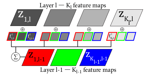
上图表示的是DN(deconvolution network的简称)的第一层，其输入图像是3通道的RGB图，学到的第一层特征有12个，说明每个输入通道图像都学习到了4个特征。而其中的特征图Z是由对应通道图像和特征分别卷积后再求和得到的。

关于卷积网络中涉及的相关计算，列出一道题比较直接：

One of the early papers on Deep Q-Learning for Atari games (Mnih et al, 2013) contains this description of its Convolutional Neural Network:
"The input to the neural network consists of an 84 × 84 × 4 image. 
The first hidden layer convolves 16   8 × 8 filters with stride 4 with the input image and applies a rectifier nonlinearity. 
The second hidden layer convolves    4 × 4 filters with stride 2, again followed by a rectifier nonlinearity. 
The final hidden layer is fully-connected and consists of  rectifier units. 
The output layer is a fully-connected linear layer with a single output for each valid action. 
The number of valid actions varied between 4 and 18 on the games we considered."
For each layer in this network, compute the number of

weights per neuron in this layer (including bias)？
neurons in this layer？
connections into the neurons in this layer？
independent parameters in this layer？
You should assume there are 18 valid actions (outputs).

First Convolutional Layer:
J = K = 84, L = 4, M = N = 8, P = 0, s = 4

weights per neuron:	    1 + M × N × L = 1 + 8 × 8 × 4 =
width and height of layer:	1+(J-M)/s = 1+(84-8)/4 =
neurons in layer:	     20 × 20 × 16 = 6400
connections:	       20 × 20 × 16 × 257 = 1644800
independent parameters:           × 257 = 4112

Second Convolutional Layer:
J = K = 20, L = 16, M = N = 4, P = 0, s = 2

weights per neuron:	1 + M × N × L = 1 + 4 × 4 × 16 = 257
width and height of layer:	1+(J-M)/s = 1+(20-4)/2 = 9
neurons in layer:	9 × 9 × 32 = 2592
connections:	9 × 9 × 32 × 257 = 666144
independent parameters:	32 × 257 = 8224
Fully Connected Layer:

weights per neuron:	1 + 2592 = 2593
neurons in layer:	256
connections:	256 × 2593 = 663808
independent parameters:	663808
Output Layer:

weights per neuron:	1 + 256 = 257
neurons in layer:	18
connections:	18 × 257 = 4626
independent parameters:	4626

链接：https://www.zhihu.com/question/43609045/answer/132235276

[1] Zeiler M D, Krishnan D, Taylor G W, etal. Deconvolutional networks[C]. Computer Vision and Pattern Recognition, 2010.
[2] Zeiler M D, Taylor G W, Fergus R, etal. Adaptive deconvolutional networks for mid and high level featurelearning[C]. International Conference on Computer Vision, 2011.
[3] Zeiler M D, Fergus R. Visualizing andUnderstanding Convolutional Networks[C]. European Conference on ComputerVision, 2013.
[4] Long J, Shelhamer E, Darrell T, et al.Fully convolutional networks for semantic segmentation[C]. Computer Vision andPattern Recognition, 2015.
[5] Unsupervised Representation Learningwith Deep Convolutional Generative Adversarial Networks
[6] Sparse Coding - Ufldl
[7] Denoising Autoencoders (dA)
[8] Convolution arithmetic tutorial

Reference

逆卷积【就是反卷积】的一个很有趣的应用是GAN(Generative Adversarial Network)里用来生成图片：Generative Models

deconv的用处挺广，涉及到visualization / pixel-wiseprediction / unsupervised learning / image generation都会用到deconv的结构。

比如Deconvolutional Network[1][2]做图片的unsupervised feature learning，ZF-Net论文中的卷积网络可视化[3]，FCN网络中的upsampling[4]，GAN中的Generative图片生成[5]。

 

Deconvolution大致可以分为以下几个方面：

1. unsupervised learning，其实就是covolutional sparse coding 卷积稀疏编码[1][2]：这里的deconv只是观念上和传统的conv反向，传统的conv是从图片生成feature map，而deconv是用unsupervised的方法找到一组kernel和feature map，让它们重建图片。
2. CNN可视化[3]：通过deconv将CNN中conv得到的feature map还原到像素空间，以观察特定的feature map对哪些pattern的图片敏感，这里的deconv其实不是conv的可逆运算，只是conv的transpose，所以tensorflow里一般取名叫transpose_conv。
3. upsampling[4][5]：在pixel-wise prediction比如image segmentation[4]以及image generation[5]中，由于需要做原始图片尺寸空间的预测，而卷积由于stride往往会降低图片size， 所以往往需要通过upsampling的方法来还原到原始图片尺寸，deconv就充当了一个upsampling的角色。

---

作者：谭旭
链接：https://www.zhihu.com/question/43609045/answer/132235276

[1. covolutional sparse coding]

第一篇文章 Deconvolutional Networks[1] 主要用于学习图片的中低层级的特征表示，

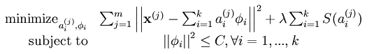
属于unsupervised feature learning，和传统的auto-encoder，RBM比较类似，和它最像的还是sparse coding，

Ref: [UFLDL] Sparse Representation

Sparse coding一个不足就是runtime cost比较高。

• learning阶段需要学习a和phi
• inference阶段还是需要学习a

接下来开始介绍Deconvolutional Network，和sparse coding的思路比较类似，

是学输入图片y的latent feature map z，同时也要学卷积核f。

如果非要用sparse coding那套来类比解释的话，就是学习图片在basis空间f的系数表示z。

只是操作由点乘变成了卷积，如下图所示，

<img src="https://pic3.zhimg.com/50/v2-adc1f9adffa771ed176ba808c0d94f22_hd.png" data-rawwidth="256" data-rawheight="102" class="content_image" width="256">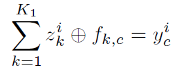

c 是图片的feature map（color channel）数量；

k 是feature map数量；

z 是feature map，【a，系数】

f 是卷积核，【phi，基】

y 是输入图片。

Loss function是：

<img src="https://pic3.zhimg.com/50/v2-5279c7bdd068c2fc29ce2826f938768e_hd.png" data-rawwidth="651" data-rawheight="113" class="origin_image zh-lightbox-thumb" width="651" data-original="https://pic3.zhimg.com/v2-5279c7bdd068c2fc29ce2826f938768e_r.png">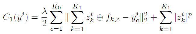

上述结构只是单层的deconvolutional layer，可以继续按照这个方法叠加layer，第一层的z就作为第二层的图片输入。Loss function如式3：

<img src="https://pic1.zhimg.com/50/v2-1ff9c78e02ea86137f0910bc45b129e4_hd.png" data-rawwidth="749" data-rawheight="215" class="origin_image zh-lightbox-thumb" width="749" data-original="https://pic1.zhimg.com/v2-1ff9c78e02ea86137f0910bc45b129e4_r.png">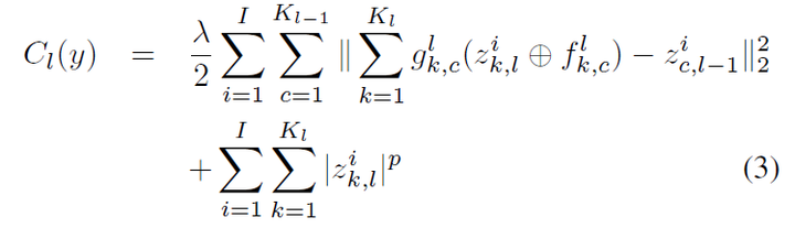

其中

<img src="https://pic3.zhimg.com/50/v2-242a3703ae5c72cf7d996f997b5ff73a_hd.png" data-rawwidth="81" data-rawheight="44" class="content_image" width="81">就是上一层的feature map表示，作为当前层的输入，

 就是上一层的feature map表示，作为当前层的输入，

<img src="https://pic2.zhimg.com/50/v2-f4aadc2f410aedd660934b82c305fe55_hd.png" data-rawwidth="61" data-rawheight="46" class="content_image" width="61">是一个0-1矩阵，相当于一个mask，用来决定哪些位置的输入需要连接，有点denoising auto-encoder的味道，附上denoising auto-encoder的关于denoising的解释[7]：

 是一个0-1矩阵，相当于一个mask，用来决定哪些位置的输入需要连接，

有点denoising auto-encoder的味道，附上denoising auto-encoder的关于denoising的解释[7]：

<img src="https://pic3.zhimg.com/50/v2-ec7c82357b96a27dd977d6cd9e84f636_hd.png" data-rawwidth="608" data-rawheight="126" class="origin_image zh-lightbox-thumb" width="608" data-original="https://pic3.zhimg.com/v2-ec7c82357b96a27dd977d6cd9e84f636_r.png">上图说明基于一部分变量去预测另一部分变量的能力是学习变量的联合分布的关键，这也是Gibbs sampling能work的原因。

 

上图说明基于一部分变量去预测另一部分变量的能力是学习变量的联合分布的关键，这也是Gibbs sampling能work的原因。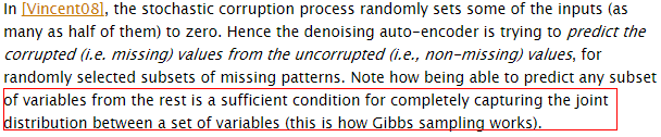

(1) learning

Deconcolutional Network的学习也是alterlative交替优化，

1. 先优化 feature map z
2. 再优化 filter f

如果有多层的话也是逐层训练。

首先第一步是学习feature map。

学习Deconcolutional Network的loss function有些困难，原因是feature map中的不同位置的点因为filter互相耦合比较严重。

作者尝试了GD，SGD，IRLS(Iterative Reweighted Least Squares)这些优化方法，效果都不理想。

因此作者使用了另外一个优化方法，不是直接优化式3中的z，而是选择了一个代理变量x，让z接近x，同时正则化x达到和式3中loss function同样的效果：

<img src="https://pic4.zhimg.com/50/v2-d1aebb4137df5c50b59f9b8e8b04da3f_hd.png" data-rawwidth="465" data-rawheight="140" class="origin_image zh-lightbox-thumb" width="465" data-original="https://pic4.zhimg.com/v2-d1aebb4137df5c50b59f9b8e8b04da3f_r.png">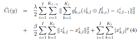

优化上式也是采用交替优化z和x的方法。

第二步是学习filter，正常的梯度下降即可。

整个Deconvolutional Network的学习算法如下图所示，其中红色框是学习feature map，其实也相当于做inference，蓝色框是学习filter，相当于模型本身的参数学习。

<img src="https://pic4.zhimg.com/50/v2-9c463735185823db0504b169b014969b_hd.png" data-rawwidth="481" data-rawheight="404" class="origin_image zh-lightbox-thumb" width="481" data-original="https://pic4.zhimg.com/v2-9c463735185823db0504b169b014969b_r.png">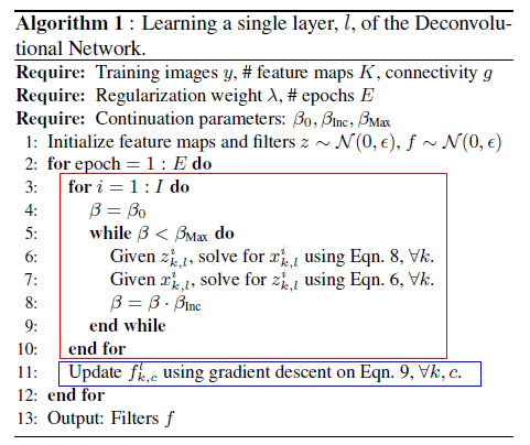

 

(2) inference

Inference包括两个层面：

第一，根据输入图片和学到的filter 从而 inference latent feature map，

第二，根据latent feature map reconstruct图片。

以两层Deconcolutional Network为例，首先学习第一层z1，然后学习第二层的z2，注意第二层的学习有两个loss，

• 一个是重建z1的loss，即project 1次学习和z1的误差

<img src="https://pic3.zhimg.com/50/v2-fa38e163127a5387f4a3941482e9f876_hd.png" data-rawwidth="406" data-rawheight="73" class="content_image" width="406">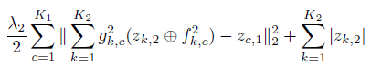　　

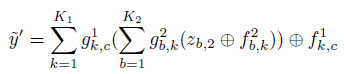
• 一个是继续重建原图片的loss，即project两次学习和原始图片y的误差

<img src="https://pic1.zhimg.com/50/v2-702ec3493d3d1d7b87291b8aa99ef32c_hd.png" data-rawwidth="498" data-rawheight="77" class="origin_image zh-lightbox-thumb" width="498" data-original="https://pic1.zhimg.com/v2-702ec3493d3d1d7b87291b8aa99ef32c_r.png">　　<img src="https://pic1.zhimg.com/50/v2-e4ac05f5f594f8733feb3e49d21cd038_hd.png" data-rawwidth="344" data-rawheight="74" class="content_image" width="344">

　　

下图是Deconcolutional Network学习到的filter示例，可以看到通过unsupervised的方法一样能学到线条以及线条组合等中低层特征，具体分析可见论文。

<img src="https://pic1.zhimg.com/50/v2-eed4e7134658a5d729e5bd39d36f9020_hd.png" data-rawwidth="468" data-rawheight="733" class="origin_image zh-lightbox-thumb" width="468" data-original="https://pic1.zhimg.com/v2-eed4e7134658a5d729e5bd39d36f9020_r.png">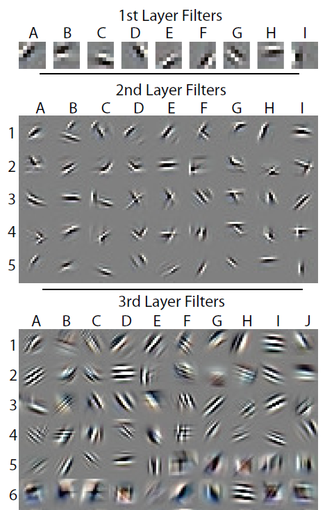

第二篇文章 Adaptive Deconvolutional Networks for Mid and High Level Feature Learning[2]也是通过deconvolutional network学习图片的特征表示，

和上一篇不同的是加入了pooling，unpooling , deconv (transpose conv，deconv的参数只是原卷积的转置，并不原卷积的可逆运算)。

这篇文章才是可视化常用的反卷积，上篇文章的deconv只是说conv的方向从feature map到图片，也还是feedforward的概念，不是这篇里用的conv和transpose conv。

这篇文章就是要学习图片的所有层级的特征，还是用unsupervised的方法。以往的其它方法在逐层学习的时候图片原始像素丢掉了，学习的target只是上一层的feature map，所以高层的filter和输入图片的连接就没那么强了，导致学得不好，所以它要end to end的学习，学习都是以原始像素作为target学习。

网络结构还是一样有deconvolution。

<img src="https://pic4.zhimg.com/50/v2-74efc1136729ec4025c1f0b77c42b143_hd.png" data-rawwidth="180" data-rawheight="71" class="content_image" width="180">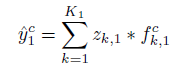

然后引入了pooling，采用的是3D pooling，both in a 2D map　and between maps，

然后记录max pooling value and switch idx，也就是pooling的receptive field中最大值的位置。

unpooling的时候最大值的位置还原，其它位置填0，如下图所示：

<img src="https://pic2.zhimg.com/50/v2-f39e054f42aa96a7daf2b783fd0e3529_hd.png" data-rawwidth="461" data-rawheight="250" class="origin_image zh-lightbox-thumb" width="461" data-original="https://pic2.zhimg.com/v2-f39e054f42aa96a7daf2b783fd0e3529_r.png">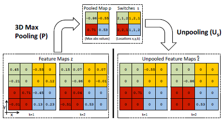

整个网络结构（两层）如下图所示：

<img src="https://pic1.zhimg.com/50/v2-29418ed101812ee96f08a8347949b848_hd.png" data-rawwidth="341" data-rawheight="614" class="content_image" width="341">

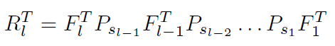
首先看右边的卷积通道：y--conv1--z1--pool1--p1--conv2--z2--pool2--p2

然后是左边的反卷积通道：p2--unpool2--z2--devonv2--p1--unpool2--z1--deconv1--y^

同一层中的conv与deconv的参数是转置关系，整个conv通道用

<img src="https://pic4.zhimg.com/50/v2-eadf811cd1e8f76815981c23333985bf_hd.png" data-rawwidth="74" data-rawheight="60" class="content_image" width="74">表示，deconv通道用

 表示，deconv通道用

<img src="https://pic1.zhimg.com/50/v2-015a6e2ec75e70dab8e27c27c19a9358_hd.png" data-rawwidth="71" data-rawheight="62" class="content_image" width="71">表示，下标l代表deconv网络的层数，conv通道的组成为：

 表示，下标l代表deconv网络的层数，conv通道的组成为：

<img src="https://pic2.zhimg.com/50/v2-a0c607fd87df5314776f1a75090caa9d_hd.png" data-rawwidth="471" data-rawheight="65" class="origin_image zh-lightbox-thumb" width="471" data-original="https://pic2.zhimg.com/v2-a0c607fd87df5314776f1a75090caa9d_r.png">

网络的学习也是分两个步骤，先固定filter学习feature map (inference)，然后固定feature map学习filter (learning)，和上一篇文章一样，学习没什么难的，大致步骤如下图，具体可以参见paper细节，

图片中的红框代表inference，蓝框代表learning。

<img src="https://pic1.zhimg.com/50/v2-e8795dc4e8537f5d02658ca7ece69b1c_hd.png" data-rawwidth="464" data-rawheight="492" class="origin_image zh-lightbox-thumb" width="464" data-original="https://pic1.zhimg.com/v2-e8795dc4e8537f5d02658ca7ece69b1c_r.png">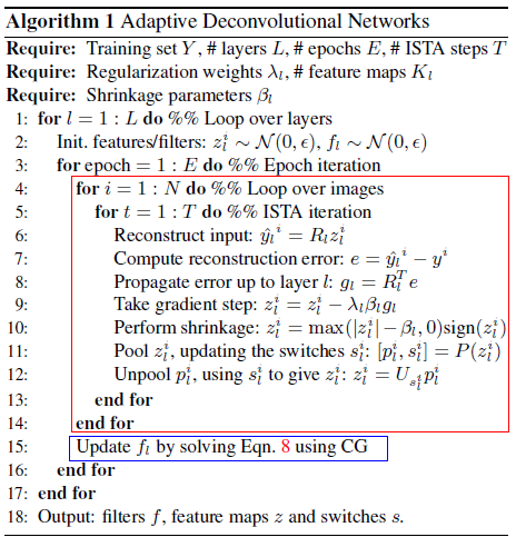

最后将提出来的feature用于图片识别分类，使用中间层的feature map作为SPM (Spatial Pyramid Matching) 的输入，M个feature map的reconstruction average 起来，得到一个SPM的single pyramid，

最后SPM分类器的效果能达到comparable的效果。

 

 

[2. CNN可视化]
deconv第二个方面是用来做CNN的可视化。

ZF-Net[3]中用到了deconv来做可视化，它是将CNN学习到的feature map用得到这些feature map的卷积核，取转置，将图片特征从feature map空间转化到pixel空间，以发现是哪些pixel激活了特定的feature map，达到分析理解CNN的目的。

 

Ref: 用TensorFlow可视化卷积层的方法

 

[3. upsampling]
分别简单介绍两篇文章，FCN和DCAN。FCN[4]主要用来做pixel-wise的image segmentation预测，先用传统的CNN结构得到feature map，同时将传统的full connected转换成了对应参数的卷积层，比如传统pool5层的尺寸是7×7×512，fc6的尺寸是4096，传统的full connected weight是7×7×512×4096这样多的参数，将它转成卷积核，kernel size为7×7，input channel为512，output channel为4096，则将传统的分别带有卷积和全连接的网络转成了全卷积网络(fully convolutional network, FCN)。FCN的一个好处是输入图片尺寸大小可以任意，不受传统网络全连接层尺寸限制，传统的方法还要用类似SPP结构来避免这个问题。FCN中为了得到pixel-wise的prediction，也要把feature map通过deconv转化到像素空间。论文中还有一些具体的feature融合，详情可参见论文。

DCGAN[5]中使用deconv就更自然了，本身GAN就需要generative model，需要通过deconv从特定分布的输入数据中生成图片。GAN这种模式被Yann LeCun特别看好，认为是unsupervised learning的一个未来。

 Jeff: 这篇文章是未来GAN系列的基础，Reference中的论文需要细啃。