课程二(Improving Deep Neural Networks: Hyperparameter tuning, Regularization and Optimization)，第一周（Practical aspects of Deep Learning） —— 4.Programming assignments:Gradient Checking

Gradient Checking

Welcome to this week's third programming assignment! You will be implementing gradient checking to make sure that your backpropagation implementation is correct. By completing this assignment you will:

- Implement gradient checking from scratch.

- Understand how to use the difference formula to check your backpropagation implementation.

- Recognize that your backpropagation algorithm should give you similar results as the ones you got by computing the difference formula.

- Learn how to identify which parameter's gradient was computed incorrectly.

Take your time to complete this assignment, and make sure you get the expected outputs when working through the different exercises. In some code blocks, you will find a "#GRADED FUNCTION: functionName" comment. Please do not modify it. After you are done, submit your work and check your results. You need to score 80% to pass. Good luck :) !

【中文翻译】

梯度检查

欢迎来到本周的第三次编程任务!您将实梯度检查, 以确保您的反向实现是正确的。通过完成此任务, 您将:

-从头开始执行梯度检查。

-了解如何使用差异公式来检查您的反向实现。

-认识到你的反向算法应该给你与计算误差公式类似的结果。

-了解如何确定哪个参数的梯度计算错误了。

 

花时间完成这项任务, 并确保在通过不同的练习时得到预期的输出。在某些代码块中, 您将找到一个 "#GRADED FUNCTION: functionName" 的注释。请不要修改它。完成后, 提交您的工作, 并检查您的结果。你需要得分80% 才能过关。祝你好运:)!

 

Gradient Checking

Welcome to the final assignment for this week! In this assignment you will learn to implement and use gradient checking.

You are part of a team working to make mobile payments available globally, and are asked to build a deep learning model to detect fraud--whenever someone makes a payment, you want to see if the payment might be fraudulent, such as if the user's account has been taken over by a hacker.

But backpropagation is quite challenging to implement, and sometimes has bugs. Because this is a mission-critical application, your company's CEO wants to be really certain that your implementation of backpropagation is correct. Your CEO says, "Give me a proof that your backpropagation is actually working!" To give this reassurance, you are going to use "gradient checking".

Let's do it!

【中文翻译】

梯度检查

欢迎来到这周的最后任务!在此作业中, 您将学习如何实现和使用梯度检查。

你是一个团队的一部分, 致力于让移动支付在全球范围内可用, 并要求建立一个深入的学习模型来检测欺诈--每当有人付款时, 你想看看付款是否可能是欺诈性的, 例如, 如果用户的帐户已被黑客接管 。

实现反向传播是相当有挑战性的， 有时有错误。因为这是一个关键任务的应用程序, 你的公司的首席执行官希望真正确定你的反向传播是正确的。你的首席执行官说, "给我一个证明, 你的反向是实际有效的!为了保证这一点, 您将使用 "梯度检查"。

让我们开始吧!

 

【code】

# Packages
import numpy as np
from testCases import *
from gc_utils import sigmoid, relu, dictionary_to_vector, vector_to_dictionary, gradients_to_vector

1) How does gradient checking work?

Backpropagation computes the gradients, where θ denotes the parameters of the model. J is computed using forward propagation and your loss function.

Because forward propagation is relatively easy to implement, you're confident you got that right, and so you're almost 100% sure that you're computing the cost J correctly. Thus, you can use your code for computing J to verify the code for computing

Let's look back at the definition of a derivative (or gradient):

If you're not familiar with the notation, it's just a way of saying "when ε is really really small."

We know the following:

•  is what you want to make sure you're computing correctly.
• You can compute J(θ+ε)and J(θ−ε) (in the case that θ is a real number), since you're confident your implementation for J is correct.

Lets use equation (1) and a small value for ε to convince your CEO that your code for computing  is correct!

2) 1-dimensional gradient checking

Consider a 1D linear function J(θ)=θx. The model contains only a single real-valued parameter(实值参数) θ, and takes x as input.

You will implement code to compute J(.)and its derivative. You will then use gradient checking to make sure your derivative computation for J is correct.

 

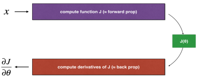
                                 Figure 1 : 1D linear model

 

The diagram above shows the key computation steps: First start with x, then evaluate the function J(x)("forward propagation"). Then compute the derivative ("backward propagation").

Exercise: implement "forward propagation" and "backward propagation" for this simple function. I.e.（即）, compute both J(.) ("forward propagation") and its derivative with respect to  ("backward propagation"), in two separate functions.

【code】

# GRADED FUNCTION: forward_propagation

def forward_propagation(x, theta):
    """
    Implement the linear forward propagation (compute J) presented in Figure 1 (J(theta) = theta * x)

    Arguments:
    x -- a real-valued input
    theta -- our parameter, a real number as well

    Returns:
    J -- the value of function J, computed using the formula J(theta) = theta * x
    """

    ### START CODE HERE ### (approx. 1 line)
    J = theta * x
    ### END CODE HERE ###

    return J

x, theta = 2, 4
J = forward_propagation(x, theta)
print ("J = " + str(J))

【result】

J = 8

Expected Output:

J

8

 

 Exercise: Now, implement the backward propagation step (derivative computation) of Figure 1. That is, compute the derivative of J(θ)=θx with respect to θ. To save you from doing the calculus, you should get 

【code】

# GRADED FUNCTION: backward_propagation

def backward_propagation(x, theta):
    """
    Computes the derivative of J with respect to theta (see Figure 1).

    Arguments:
    x -- a real-valued input
    theta -- our parameter, a real number as well

    Returns:
    dtheta -- the gradient of the cost with respect to theta
    """

    ### START CODE HERE ### (approx. 1 line)
    dtheta = x
    ### END CODE HERE ###

    return dtheta

x, theta = 2, 4
dtheta = backward_propagation(x, theta)
print ("dtheta = " + str(dtheta))

【result】

dtheta = 2

Expected Output:

dtheta

2

 

 Exercise: To show that the backward_propagation() function is correctly computing the gradient let's implement gradient checking.

Instructions:

• First compute "gradapprox" using the formula above (1) and a small value of ε. Here are the Steps to follow:

 

• Then compute the gradient using backward propagation, and store the result in a variable "grad"
• Finally, compute the relative difference between "gradapprox" and the "grad" using the following formula:

• You will need 3 Steps to compute this formula:
  • 1'. compute the numerator(分子) using np.linalg.norm(...)
  • 2'. compute the denominator（分母）. You will need to call np.linalg.norm(...) twice.
  • 3'. divide them.
• If this difference is small (say less than 10⁻⁷), you can be quite confident that you have computed your gradient correctly. Otherwise, there may be a mistake in the gradient computation.

【code】

# GRADED FUNCTION: gradient_check

def gradient_check(x, theta, epsilon = 1e-7):
    """
    Implement the backward propagation presented in Figure 1.

    Arguments:
    x -- a real-valued input
    theta -- our parameter, a real number as well
    epsilon -- tiny shift to the input to compute approximated gradient with formula(1)

    Returns:
    difference -- difference (2) between the approximated gradient and the backward propagation gradient
    """

    # Compute gradapprox using left side of formula (1). epsilon is small enough, you don't need to worry about the limit.
    ### START CODE HERE ### (approx. 5 lines)
    thetaplus = theta + epsilon                             # Step 1
    thetaminus = theta - epsilon                            # Step 2
    J_plus =  thetaplus * x                         # Step 3
    J_minus = thetaminus * x                        # Step 4
    gradapprox =( J_plus - J_minus)/ (2*epsilon )           # Step 5
    ### END CODE HERE ###

    # Check if gradapprox is close enough to the output of backward_propagation()
    ### START CODE HERE ### (approx. 1 line)
    grad = backward_propagation(x, theta)### END CODE HERE ###

    ### START CODE HERE ### (approx. 1 line)
    numerator = np.linalg.norm(grad -  gradapprox)   # Step 1' numpy.linalg.norm的用法：https://docs.scipy.org/doc/numpy/reference/generated/numpy.linalg.norm.html
    denominator =np.linalg.norm(grad)+np.linalg.norm( gradapprox)     # Step 2'
    difference =  numerator/ denominator                              # Step 3'
    ### END CODE HERE ###

    if difference < 1e-7:
        print ("The gradient is correct!")
    else:
        print ("The gradient is wrong!")

    return difference

x, theta = 2, 4
difference = gradient_check(x, theta)
print("difference = " + str(difference))

【result】

The gradient is correct!
difference = 2.91933588329e-10

Expected Output: The gradient is correct!

difference

2.9193358103083e-10

Congrats, the difference is smaller than the 10⁻⁷ threshold. So you can have high confidence that you've correctly computed the gradient in backward_propagation().

Now, in the more general case, your cost function J has more than a single 1D input. When you are training a neural network, θ actually consists of multiple matrices W^[l] and biases b^[l]! It is important to know how to do a gradient check with higher-dimensional inputs. Let's do it!

3) N-dimensional gradient checking

 

The following figure describes the forward and backward propagation of your fraud detection (欺诈检验) model.

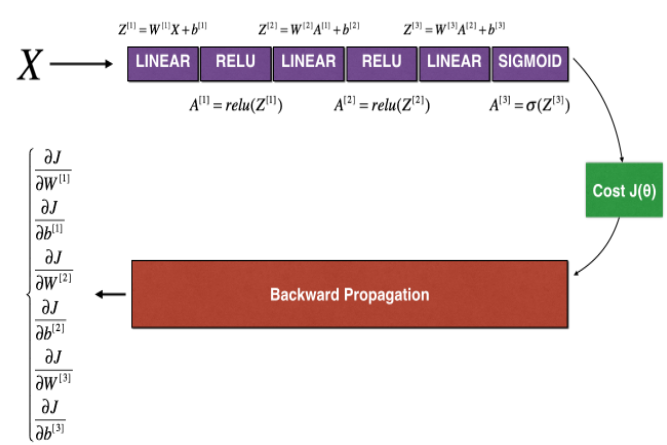
                                            Figure 2 : deep neural network
                         LINEAR -> RELU -> LINEAR -> RELU -> LINEAR -> SIGMOID

Let's look at your implementations （实现） for forward propagation and backward propagation.

【code】

def forward_propagation_n(X, Y, parameters):
    """
    Implements the forward propagation (and computes the cost) presented in Figure 2.

    Arguments:
    X -- training set for m examples
    Y -- labels for m examples
    parameters -- python dictionary containing your parameters "W1", "b1", "W2", "b2", "W3", "b3":
                    W1 -- weight matrix of shape (5, 4)
                    b1 -- bias vector of shape (5, 1)
                    W2 -- weight matrix of shape (3, 5)
                    b2 -- bias vector of shape (3, 1)
                    W3 -- weight matrix of shape (1, 3)
                    b3 -- bias vector of shape (1, 1)

    Returns:
    cost -- the cost function (logistic cost for one example)
    """

    # retrieve （检索）parameters
    m = X.shape[1]
    W1 = parameters["W1"]
    b1 = parameters["b1"]
    W2 = parameters["W2"]
    b2 = parameters["b2"]
    W3 = parameters["W3"]
    b3 = parameters["b3"]

    # LINEAR -> RELU -> LINEAR -> RELU -> LINEAR -> SIGMOID
    Z1 = np.dot(W1, X) + b1
    A1 = relu(Z1)
    Z2 = np.dot(W2, A1) + b2
    A2 = relu(Z2)
    Z3 = np.dot(W3, A2) + b3
    A3 = sigmoid(Z3)

    # Cost
    logprobs = np.multiply(-np.log(A3),Y) + np.multiply(-np.log(1 - A3), 1 - Y)
    cost = 1./m * np.sum(logprobs)

    cache = (Z1, A1, W1, b1, Z2, A2, W2, b2, Z3, A3, W3, b3)

    return cost, cache

Now, run backward propagation.

def backward_propagation_n(X, Y, cache):
    """
    Implement the backward propagation presented in figure 2.

    Arguments:
    X -- input datapoint, of shape (input size, 1)
    Y -- true "label"
    cache -- cache output from forward_propagation_n()

    Returns:
    gradients -- A dictionary with the gradients of the cost with respect to each parameter, activation and pre-activation variables.
    """

    m = X.shape[1]
    (Z1, A1, W1, b1, Z2, A2, W2, b2, Z3, A3, W3, b3) = cache

    dZ3 = A3 - Y
    dW3 = 1./m * np.dot(dZ3, A2.T)
    db3 = 1./m * np.sum(dZ3, axis=1, keepdims = True)

    dA2 = np.dot(W3.T, dZ3)
    dZ2 = np.multiply(dA2, np.int64(A2 > 0))
    dW2 = 1./m * np.dot(dZ2, A1.T) * 2   # ？？？ 此处有错误,应该为 dW2 = 1./m * np.dot(dZ2, A1.T) 
    db2 = 1./m * np.sum(dZ2, axis=1, keepdims = True)

    dA1 = np.dot(W2.T, dZ2)
    dZ1 = np.multiply(dA1, np.int64(A1 > 0))
    dW1 = 1./m * np.dot(dZ1, X.T)
    db1 = 4./m * np.sum(dZ1, axis=1, keepdims = True) # ？？？ 此处有错误,应该为  db1 = 1./m * np.sum(dZ1, axis=1, keepdims = True)

    gradients = {"dZ3": dZ3, "dW3": dW3, "db3": db3,
                 "dA2": dA2, "dZ2": dZ2, "dW2": dW2, "db2": db2,
                 "dA1": dA1, "dZ1": dZ1, "dW1": dW1, "db1": db1}

    return gradients

You obtained some results on the fraud detection test set but you are not 100% sure of your model. Nobody's perfect! Let's implement gradient checking to verify if your gradients are correct.

How does gradient checking work?.

As in 1) and 2), you want to compare "gradapprox" to the gradient computed by backpropagation. The formula is still:

However, θ is not a scalar anymore. It is a dictionary called "parameters". We implemented a function "dictionary_to_vector()" for you. It converts the "parameters" dictionary into a vector called "values", obtained by reshaping all parameters (W1, b1, W2, b2, W3, b3) into vectors and concatenating them(通过将所有参数 (W1、b1、W2、b2、W3、b3) 重新整形, 并将它们串联起来。).

The inverse function is "vector_to_dictionary" which outputs back the "parameters" dictionary.

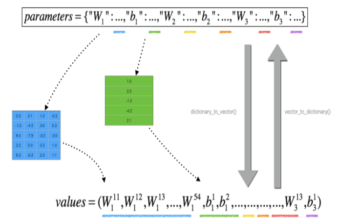
                    Figure 2 : dictionary_to_vector() and vector_to_dictionary()
                        You will need these functions in gradient_check_n()

We have also converted the "gradients" dictionary into a vector "grad" using gradients_to_vector(). You don't need to worry about that.

Exercise: Implement gradient_check_n().

Instructions: Here is pseudo-code(伪代码) that will help you implement the gradient check.

For each i in num_parameters:

Thus, you get a vector gradapprox, where gradapprox[i] is an approximation of the gradient with respect to parameter_values[i]. You can now compare this gradapprox vector to the gradients vector from backpropagation. Just like for the 1D case (Steps 1', 2', 3'), compute:

【code】

# GRADED FUNCTION: gradient_check_n

def gradient_check_n(parameters, gradients, X, Y, epsilon = 1e-7):
    """
    Checks if backward_propagation_n computes correctly the gradient of the cost output by forward_propagation_n

    Arguments:
    parameters -- python dictionary containing your parameters "W1", "b1", "W2", "b2", "W3", "b3":
    grad -- output of backward_propagation_n, contains gradients of the cost with respect to the parameters.
    X -- input datapoint, of shape (input size, 1)
    Y -- true "label"
    epsilon -- tiny shift to the input to compute approximated gradient with formula(1)

    Returns:
    difference -- difference (2) between the approximated gradient and the backward propagation gradient
    """

    # Set-up variables
    parameters_values, _ = dictionary_to_vector(parameters)
    grad = gradients_to_vector(gradients)
    num_parameters = parameters_values.shape[0]  # ？？？   num_parameters应该是列向量，图2中是行向量
    J_plus = np.zeros((num_parameters, 1))
    J_minus = np.zeros((num_parameters, 1))
    gradapprox = np.zeros((num_parameters, 1))

    # Compute gradapprox
    for i in range(num_parameters):

        # Compute J_plus[i]. Inputs: "parameters_values, epsilon". Output = "J_plus[i]".
        # "_" is used because the function you have to outputs two parameters but we only care about the first one
        ### START CODE HERE ### (approx. 3 lines)
        thetaplus = np.copy(parameters_values)                                      # Step 1
        thetaplus[i][0] = thetaplus[i][0]+ epsilon                                  # Step 2
        J_plus[i], _ = forward_propagation_n(X, Y, vector_to_dictionary( thetaplus ))   # Step 3
        ### END CODE HERE ###

        # Compute J_minus[i]. Inputs: "parameters_values, epsilon". Output = "J_minus[i]".
        ### START CODE HERE ### (approx. 3 lines)
        thetaminus =  np.copy(parameters_values)                                     # Step 1
        thetaminus[i][0] =  thetaminus[i][0]- epsilon                             # Step 2
        J_minus[i], _ = forward_propagation_n(X, Y, vector_to_dictionary(  thetaminus ))     # Step 3
        ### END CODE HERE ###

        # Compute gradapprox[i]
        ### START CODE HERE ### (approx. 1 line)
        gradapprox[i] = ( J_plus[i]- J_minus[i])/ (2*epsilon )
        ### END CODE HERE ###

    # Compare gradapprox to backward propagation gradients by computing difference.
    ### START CODE HERE ### (approx. 1 line)
    numerator =  np.linalg.norm(grad -  gradapprox)                     # Step 1'
    denominator = np.linalg.norm(grad)+np.linalg.norm( gradapprox)      # Step 2'
    difference =numerator /  denominator                               # Step 3'
    ### END CODE HERE ###

    if difference > 2e-7:
        print ("\033[93m" + "There is a mistake in the backward propagation! difference = " + str(difference) + "\033[0m")
    else:
        print ("\033[92m" + "Your backward propagation works perfectly fine! difference = " + str(difference) + "\033[0m")

    return difference

X, Y, parameters = gradient_check_n_test_case()

cost, cache = forward_propagation_n(X, Y, parameters)
gradients = backward_propagation_n(X, Y, cache)
difference = gradient_check_n(parameters, gradients, X, Y)

【result】

here is a mistake in the backward propagation! difference = 0.285093156781

Expected output:

There is a mistake in the backward propagation!

difference = 0.285093156781

It seems that there were errors in the backward_propagation_n code we gave you! Good that you've implemented the gradient check. Go back to backward_propagation and try to find/correct the errors (Hint: check dW2 and db1). Rerun the gradient check when you think you've fixed it. Remember you'll need to re-execute the cell defining backward_propagation_n() if you modify the code.

Can you get gradient check to declare your derivative computation correct? Even though this part of the assignment isn't graded, we strongly urge you to try to find the bug and re-run gradient check until you're convinced backprop is now correctly implemented.

Note

• Gradient Checking is slow! Approximating (逼近)the gradient with 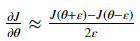is computationally costly. For this reason, we don't run gradient checking at every iteration during training. Just a few times to check if the gradient is correct.
• Gradient Checking, at least as we've presented it（至少正如我们所介绍的）, doesn't work with dropout. You would usually run the gradient check algorithm without dropout to make sure your backprop is correct, then add dropout.

Congrats, you can be confident that your deep learning model for fraud detection is working correctly! You can even use this to convince your CEO. :)

What you should remember from this notebook:

• Gradient checking verifies closeness between the gradients from backpropagation and the numerical approximation of the gradient (computed using forward propagation).
• Gradient checking is slow, so we don't run it in every iteration of training. You would usually run it only to make sure your code is correct, then turn it off and use backprop for the actual learning process.

【中文翻译】

您应该记住的：

　　梯度检查验证反向传播过程中计算的导数和数值逼近得到的导数 (使用向前传播计算) 之间的距离。

　　梯度检查很慢, 所以我们不在每次训练的迭代中都运行它。您通常只运行它, 以确保您的代码是正确的, 然后关闭它, 并使用 backprop，进行实际的训练。