TensorFlow.NET机器学习入门【7】采用卷积神经网络(CNN)处理Fashion-MNIST
本文将介绍如何采用卷积神经网络(CNN)来处理Fashion-MNIST数据集。
程序流程如下:
1、准备样本数据
2、构建卷积神经网络模型
3、网络学习(训练)
4、消费、测试
除了网络模型的构建,其它步骤都和前面介绍的普通神经网络的处理完全一致,本文就不重复介绍了,重点讲一下模型的构建。
先看代码:
        /// <summary>

        /// 构建网络模型

        /// </summary>

        private Model BuildModel()

        {

            // 网络参数

            float scale = 1.0f / 255;

            var model = keras.Sequential(new List<ILayer>

            {

                keras.layers.Rescaling(scale, input_shape: (img_rows, img_cols, channel)),

                keras.layers.Conv2D(32, 5, padding: "same", activation: keras.activations.Relu),

                keras.layers.MaxPooling2D(),

                keras.layers.Conv2D(64, 3, padding: "same", activation: keras.activations.Relu),

                keras.layers.MaxPooling2D(),

                keras.layers.Flatten(),

                keras.layers.Dense(128, activation: keras.activations.Relu),

                keras.layers.Dense(num_classes,activation:keras.activations.Softmax)

            });

            return model;

        }
keras.layers.Conv2D方法创建一个卷积层
keras.layers.MaxPooling2D方法创建一个池化层
卷积层的含义:
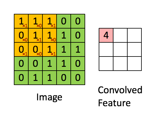
如上图所示,原始数据尺寸为5*5,卷积核大小为3*3,当卷积核滑过原始图片时,卷积核和图片对应的数据进行运算(先乘后加),并形成新的数据。
示例的卷积核为[[1,0,1],[0,1,0],[1,0,1]],和左上角数据卷积后结果为4,填写到对应位置。对整改图片全部滑动一遍,即形成最终结果。

采用卷积神经网络,相对于前面介绍的普通神经网络有什么优势呢?
1、首先,图像本身是一个二维数据,普通网络首先要把数据拉平,这一点就不合理,而卷积网络通过卷积核处理数据,保留了原始数据的基本特征;
2、其次,采用卷积网络大大减小了参数的数量。假设原始图片分辨率为100*100,拉平后长度为10000,后面跟一个全连接层,输出为128,此时参数量为(10000+1)*128,超过128万。这才一个全连接层。如果采用CNN,参数数量取决于卷积核的大小和数量。假设卷积核大小为5*5,数量为32,此时参数数量为:(5*5+1)*32=832。【计算方法下面会详细介绍】
池化层的含义:
池化就是压缩,就是图片数据太大了,通过池化把分辨率减小一些。
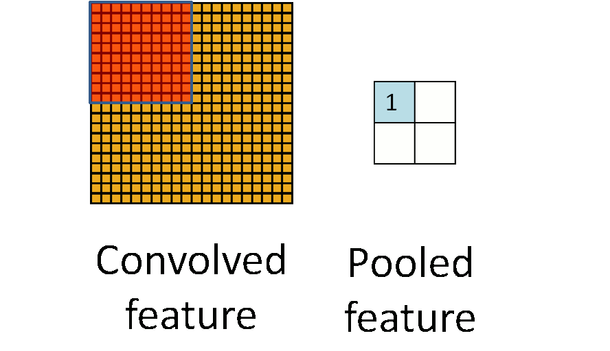
池化有均值池化和最大值池化方法,这个很好理解,就是一推数据中取平均值或最大值。MaxPooling2D明显是最大池化法。
我们再看一下这个代码:
keras.layers.Conv2D(32, 5, padding: "same", activation: keras.activations.Relu),
32表示卷积核数量为32,卷积核大小为5*5,padding: "same"表示对图像进行边缘补零,不然卷积后的图像尺寸会变小,补零后图像尺寸不变。
整体模型摘要信息如下:

下面逐行解释一下:
1、首先输入层的数据Shape为:(28,28,1),28表示图片像素,1表示灰度图片,如果是彩色图片,应该为(28,28,3)
2、Rescaling对数据进行处理,统一乘以一个系数,这里没有需要训练的参数
3、引入一个卷积层,卷积核数量为32,卷积核大小为5*5(图上看不出来),此时参数数量为:(5*5+1)*32=832,这里卷积核尺寸为5*5,所以有25个参数,这很好理解,+1是因为作为卷积计算后还要加一个偏置b,所以每个卷积核共26个参数。由于有32个卷积核,要对同一个图像采用不同的卷积核做32次计算,所以这一层输出数据为(28,28,32)
4、池化层将数据从(28,28,32)压缩到(14,14,32)
5、再引入一个卷积层,卷积核数量为64,卷积核大小为3*3(图上看不出来),这次计算和第一次不太一样:由于上一层数据共有32片,对每一片数据采用的卷积核是不一样的,所以这里实际一共有32*9=288个卷积核。首先用32个卷积核和上述32片数据分别进行卷积形成32片数据,然后将32片数据叠加求和,最后再加一个偏置形成一片新数据,重复进行64次,形成64片新数据。此时参数数量为:(288+1)*64=18496
【注意:这里的算法其实是和第一层卷积算法完全一样的,只是第一层输入为灰度图片,数据只有一片,如果输入为彩色图片,就一致了。】
6、池化层将数据从(14,14,64)压缩到(7,7,64)
7、将数据拉平,拉平后的数据长度为:7*7*64=3136
8、引入全连接层,输出神经元数量为128,此时参数数量为:(3136+1)*128=401536
9、最后为全连接层输出,输出神经元数量为10,参数数量为:(128+1)*10=1290
现在,由于参数数量已经很多了,训练需要的时间也比较长了,所以需要把训练完成后的参数保存下来,下次可以重新加载保存的参数接着训练,不用从头再来。
保存的模型也可以发布到生产系统用于实际的消费。
全部代码如下:


    /// <summary>

    /// 采用卷积神经网络处理Fashion-MNIST数据集

    /// </summary>

    public class CNN_Fashion_MNIST

    {

        private readonly string TrainImagePath = @"D:\Study\Blogs\TF_Net\Asset\fashion_mnist_png\train";

        private readonly string TestImagePath = @"D:\Study\Blogs\TF_Net\Asset\fashion_mnist_png\test";

        private readonly string train_date_path = @"D:\Study\Blogs\TF_Net\Asset\fashion_mnist_png\cnn_train_data.bin";

        private readonly string train_label_path = @"D:\Study\Blogs\TF_Net\Asset\fashion_mnist_png\cnn_train_label.bin";

        private readonly string ModelFile = @"D:\Study\Blogs\TF_Net\Model\cnn_fashion_mnist.h5";

        private readonly int img_rows = 28;

        private readonly int img_cols = 28;

        private readonly int channel = 1;

        private readonly int num_classes = 10;  // total classes

        public void Run()

        {

            var model = BuildModel();

            model.summary();

            model.load_weights(ModelFile);

            Console.WriteLine("press any key");

            Console.ReadKey();

            model.compile(optimizer: keras.optimizers.Adam(0.0001f),

                loss: keras.losses.SparseCategoricalCrossentropy(),

                metrics: new[] { "accuracy" });

            (NDArray train_x, NDArray train_y) = LoadTrainingData();

            model.fit(train_x, train_y, batch_size: 512, epochs: 1);

            model.save_weights(ModelFile);

            test(model);

        }

        /// <summary>

        /// 构建网络模型

        /// </summary>

        private Model BuildModel()

        {

            // 网络参数

            float scale = 1.0f / 255;

            var model = keras.Sequential(new List<ILayer>

            {

                keras.layers.Rescaling(scale, input_shape: (img_rows, img_cols, channel)),

                keras.layers.Conv2D(32, 5, padding: "same", activation: keras.activations.Relu),

                keras.layers.MaxPooling2D(),

                keras.layers.Conv2D(64, 3, padding: "same", activation: keras.activations.Relu),

                keras.layers.MaxPooling2D(),

                keras.layers.Flatten(),

                keras.layers.Dense(128, activation: keras.activations.Relu),

                keras.layers.Dense(num_classes,activation:keras.activations.Softmax)

            });

            return model;

        }

        /// <summary>

        /// 加载训练数据

        /// </summary>

        /// <param name="total_size"></param>

        private (NDArray, NDArray) LoadTrainingData()

        {

            try

            {

                Console.WriteLine("Load data");

                IFormatter serializer = new BinaryFormatter();

                FileStream loadFile = new FileStream(train_date_path, FileMode.Open, FileAccess.Read);

                float[,,,] arrx = serializer.Deserialize(loadFile) as float[,,,];

                loadFile = new FileStream(train_label_path, FileMode.Open, FileAccess.Read);

                int[] arry = serializer.Deserialize(loadFile) as int[];

                Console.WriteLine("Load data success");

                return (np.array(arrx), np.array(arry));

            }

            catch (Exception ex)

            {

                Console.WriteLine($"Load data Exception:{ex.Message}");

                return LoadRawData();

            }

        }

        private (NDArray, NDArray) LoadRawData()

        {

            Console.WriteLine("LoadRawData");

            int total_size = 60000;

            float[,,,] arrx = new float[total_size, img_rows, img_cols, channel];

            int[] arry = new int[total_size];

            int count = 0;

            DirectoryInfo RootDir = new DirectoryInfo(TrainImagePath);

            foreach (var Dir in RootDir.GetDirectories())

            {

                foreach (var file in Dir.GetFiles("*.png"))

                {

                    Bitmap bmp = (Bitmap)Image.FromFile(file.FullName);

                    if (bmp.Width != img_cols || bmp.Height != img_rows)

                    {

                        continue;

                    }

                    for (int row = 0; row < img_rows; row++)

                        for (int col = 0; col < img_cols; col++)

                        {

                            var pixel = bmp.GetPixel(col, row);

                            int val = (pixel.R + pixel.G + pixel.B) / 3;

                            arrx[count, row, col, 0] = val;

                            arry[count] = int.Parse(Dir.Name);

                        }

                    count++;

                }

                Console.WriteLine($"Load image data count={count}");

            }

            Console.WriteLine("LoadRawData finished");

            //Save Data

            Console.WriteLine("Save data");

            IFormatter serializer = new BinaryFormatter();

            //开始序列化

            FileStream saveFile = new FileStream(train_date_path, FileMode.Create, FileAccess.Write);

            serializer.Serialize(saveFile, arrx);

            saveFile.Close();

            saveFile = new FileStream(train_label_path, FileMode.Create, FileAccess.Write);

            serializer.Serialize(saveFile, arry);

            saveFile.Close();

            Console.WriteLine("Save data finished");

            return (np.array(arrx), np.array(arry));

        }

        /// <summary>

        /// 消费模型

        /// </summary>

        private void test(Model model)

        {

            Random rand = new Random(1);

            DirectoryInfo TestDir = new DirectoryInfo(TestImagePath);

            foreach (var ChildDir in TestDir.GetDirectories())

            {

                Console.WriteLine($"Folder:【{ChildDir.Name}】");

                var Files = ChildDir.GetFiles("*.png");

                for (int i = 0; i < 10; i++)

                {

                    int index = rand.Next(1000);

                    var image = Files[index];

                    var x = LoadImage(image.FullName);

                    var pred_y = model.Apply(x);

                    var result = argmax(pred_y[0].numpy());

                    Console.WriteLine($"FileName:{image.Name}\tPred:{result}");

                }

            }

        }

        private NDArray LoadImage(string filename)

        {

            float[,,,] arrx = new float[1, img_rows, img_cols, channel];

            Bitmap bmp = (Bitmap)Image.FromFile(filename);

            for (int row = 0; row < img_rows; row++)

                for (int col = 0; col < img_cols; col++)

                {

                    var pixel = bmp.GetPixel(col, row);

                    int val = (pixel.R + pixel.G + pixel.B) / 3;

                    arrx[0, row, col, 0] = val;

                }

            return np.array(arrx);

        }

        private int argmax(NDArray array)

        {

            var arr = array.reshape(-1);

            float max = 0;

            for (int i = 0; i < 10; i++)

            {

                if (arr[i] > max)

                {

                    max = arr[i];

                }

            }

            for (int i = 0; i < 10; i++)

            {

                if (arr[i] == max)

                {

                    return i;

                }

            }

            return 0;

        }

    }
通过采用CNN的方法,我们可以把Fashion-MNIST识别率提高到大约94%左右,而且还有提高的空间。但是网络的优化是一件非常困难的事情,特别是识别率已经很高的时候,想提高1个百分点都是很不容易的。
以下是一个优化过的网络,我查阅了不少资料,也参考了很多代码,才构建了这个网络,它的识别率约为96%,再怎么调整也提高不上去了。
        /// <summary>

        /// 构建网络模型

        /// </summary>

        private Model BuildModel()

        {

            // 网络参数

            float scale = 1.0f / 255;

            var model = keras.Sequential(new List<ILayer>

            {

                keras.layers.Rescaling(scale, input_shape: (img_rows, img_cols, channel)),

                keras.layers.Conv2D(32, 3, padding: "same", activation: keras.activations.Relu),

                keras.layers.MaxPooling2D(),

                keras.layers.Conv2D(64, 3, padding: "same", activation: keras.activations.Relu),

                keras.layers.MaxPooling2D(),

                keras.layers.Dropout(0.3f),

                keras.layers.BatchNormalization(),

                keras.layers.Conv2D(128, 3, padding: "same", activation: keras.activations.Relu),

                keras.layers.Conv2D(128, 3, padding: "same", activation: keras.activations.Relu),

                keras.layers.MaxPooling2D(),

                keras.layers.Dropout(0.4f),

                keras.layers.Flatten(),

                keras.layers.Dense(512, activation: keras.activations.Relu),

                keras.layers.Dropout(0.25f),

                keras.layers.Dense(num_classes,activation:keras.activations.Softmax)

            });

            return model;

        }
【参考资料】
卷积神经网络CNN总结 - Madcola - 博客园 (cnblogs.com)
卷积神经网络(CNN)模型结构 - 刘建平Pinard - 博客园 (cnblogs.com)
【相关资源】
源码:Git: https://gitee.com/seabluescn/tf_not.git
项目名称:CNN_Fashion_MNIST,CNN_Fashion_MNIST_Plus
TensorFlow.NET机器学习入门【7】采用卷积神经网络(CNN)处理Fashion-MNIST的更多相关文章
- 深度学习:Keras入门(二)之卷积神经网络(CNN)
说明:这篇文章需要有一些相关的基础知识,否则看起来可能比较吃力. 1.卷积与神经元 1.1 什么是卷积? 简单来说,卷积(或内积)就是一种先把对应位置相乘然后再把结果相加的运算.(具体含义或者数学公式 ...
- 深度学习:Keras入门(二)之卷积神经网络(CNN)【转】
本文转载自:https://www.cnblogs.com/lc1217/p/7324935.html 说明:这篇文章需要有一些相关的基础知识,否则看起来可能比较吃力. 1.卷积与神经元 1.1 什么 ...
- 深度学习:Keras入门(二)之卷积神经网络(CNN)(转)
转自http://www.cnblogs.com/lc1217/p/7324935.html 1.卷积与神经元 1.1 什么是卷积? 简单来说,卷积(或内积)就是一种先把对应位置相乘然后再把结果相加的 ...
- TensorFlow实战第八课(卷积神经网络CNN)
首先我们来简单的了解一下什么是卷积神经网路(Convolutional Neural Network) 卷积神经网络是近些年逐步兴起的一种人工神经网络结构, 因为利用卷积神经网络在图像和语音识别方面能 ...
- 使用卷积神经网络CNN训练识别mnist
算的的上是自己搭建的第一个卷积神经网络.网络结构比较简单. 输入为单通道的mnist数据集.它是一张28*28,包含784个特征值的图片 我们第一层输入,使用5*5的卷积核进行卷积,输出32张特征图, ...
- 卷积神经网络(CNN)代码实现(MNIST)解析
在http://blog.csdn.net/fengbingchun/article/details/50814710中给出了CNN的简单实现,这里对每一步的实现作个说明: 共7层:依次为输入层.C1 ...
- 【深度学习系列】手写数字识别卷积神经--卷积神经网络CNN原理详解(一)
上篇文章我们给出了用paddlepaddle来做手写数字识别的示例,并对网络结构进行到了调整,提高了识别的精度.有的同学表示不是很理解原理,为什么传统的机器学习算法,简单的神经网络(如多层感知机)都可 ...
- 【深度学习系列】卷积神经网络CNN原理详解(一)——基本原理
上篇文章我们给出了用paddlepaddle来做手写数字识别的示例,并对网络结构进行到了调整,提高了识别的精度.有的同学表示不是很理解原理,为什么传统的机器学习算法,简单的神经网络(如多层感知机)都可 ...
- TensorFlow.NET机器学习入门【6】采用神经网络处理Fashion-MNIST
"如果一个算法在MNIST上不work,那么它就根本没法用:而如果它在MNIST上work,它在其他数据上也可能不work". -- 马克吐温 上一篇文章我们实现了一个MNIST手 ...
随机推荐
- day16 Linux三剑客之awk
day16 Linux三剑客之awk 1.什么是awk,主要作用是什么? 什么是awk,主要作用是什么? awk 主要用来处理文件,将文本按照指定的格式输出.其中包含变量,循环以及数组. 2.awk的 ...
- Flink基础
一.抽象层次 Flink提供不同级别的抽象来开发流/批处理应用程序. 最低级抽象只提供有状态流.它 通过Process Function嵌入到DataStream API中.它允许用户自由处理来自 ...
- windows Visual Studio 上安装 CUDA【转载】
原文 : http://blog.csdn.net/augusdi/article/details/12527497 前提安装: Visual Studio 2012 Visual Assist X ...
- android知识点duplicateParentState
android知识点duplicateParentState 今天要做一个效果,组件RelativeLayout上有两个TextView,这两个TextView具有不同的颜色值,现在要的效果是,当Re ...
- Linux基础命令---mailq显示邮件队列
mailq mailq指令可以显示出待发送的邮件队列. 此命令的适用范围:RedHat.RHEL.Ubuntu.CentOS.Fedora. 1.语法 mailq 2.选项参数列表 ...
- Output of C++ Program | Set 5
Difficulty Level: Rookie Predict the output of below C++ programs. Question 1 1 #include<iostream ...
- 【手帐】Bullet Journal教程
最近觉得自己的日程记录本有待提高,于是从今年开始开始入坑了手帐. *内容源自Bullet Journal官网.https://bulletjournal.com/pages/learn 快速笔记 Bu ...
- SharedWorker实现多标签页联动计时器
web workers对于每个前端开发者并不陌生,在mdn中的定义:Web Worker为Web内容在后台线程中运行脚本提供了一种简单的方法.线程可以执行任务而不干扰用户界面.此外,他们可以使用XML ...
- shell脚本 系统状态信息查看
一.简介 源码地址 日期:2018/6/23 介绍:显示简单的系统信息 效果图: 二.使用 适用:centos6+,ubuntu12+ 语言:中文 注意:无 下载 wget https://raw.g ...
- 日程表(Project)
<Project2016 企业项目管理实践>张会斌 董方好 编著 Project默认打开时,在功能区下面会有一个[日程表],如果不见了,那肯定里什么时候手贱关掉的,不要紧,还可以到[视图] ...