《FDTD electromagnetic field using MATLAB》读书笔记之 Figure 1.14

背景：

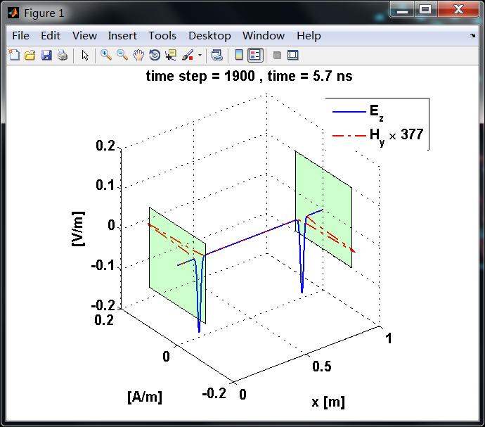
基于公式1.42（Ez分量）、1.43（Hy分量）的1D FDTD实现。

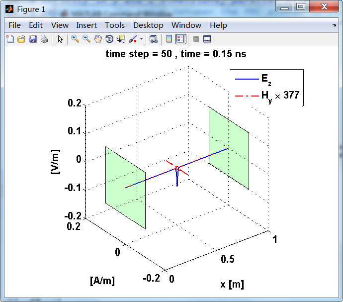
计算电场和磁场分量，该分量由z方向的电流片Jz产生，Jz位于两个理想导体极板中间，两个极板平行且向y和z方向无限延伸。

          平行极板相距1m，差分网格Δx=1mm。

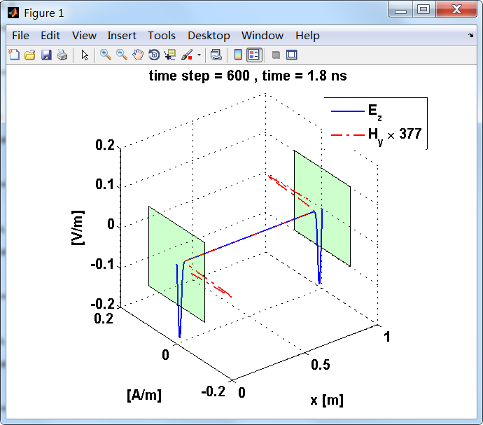
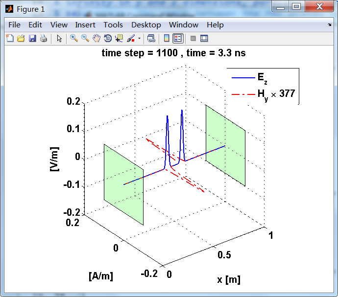
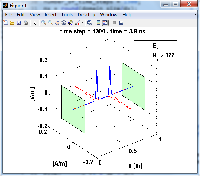
电流面密度导致分界面（电流薄层）磁场分量的不连续，在两侧产生Hy的波，每个强度为5×10^（-4）A/m。因为电磁波在自由空间中传播，本征阻抗为η0。

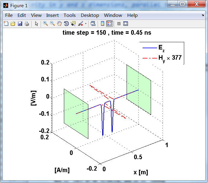
          显示了从左右极板反射前后的传播过程。本例中是PEC边界，正切电场分量（Ez）在PEC表面消失。

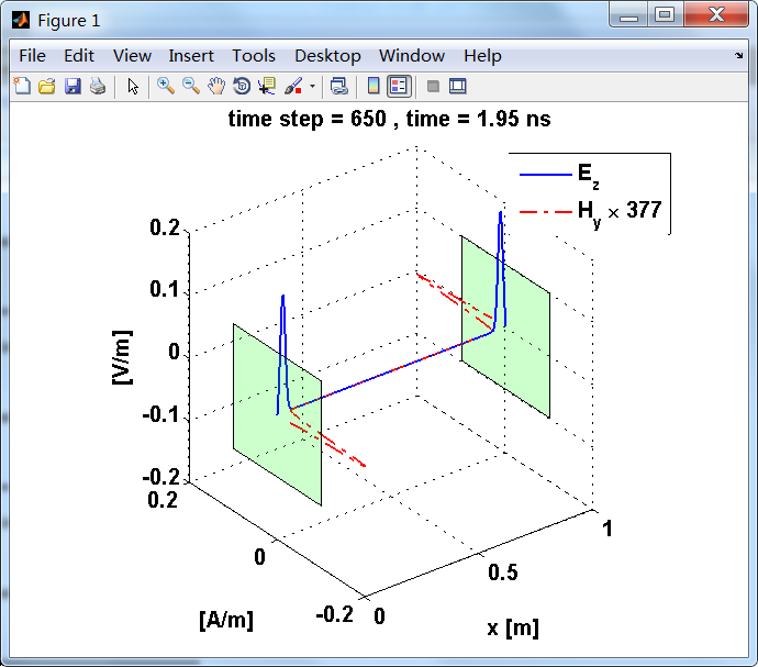
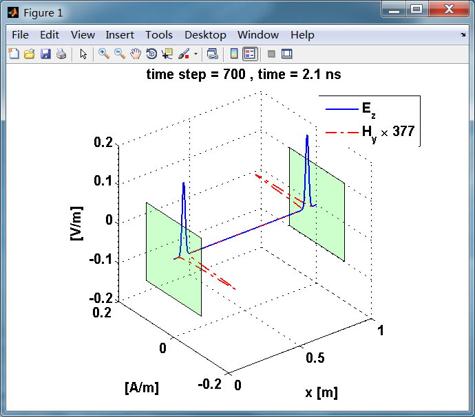
观察图中step650到700的场的变换情况，经过PEC板的入射波和反射波的传播特征。经过PEC反射后，Ez的极性变反，这是因为反射系数等于-1；

而磁场分量Hy没有反向，反射系数等于1。

下面是书中的代码（几乎没动）：

第1个是主程序：

%% ------------------------------------------------------------------------------
%%            Output Info about this m-file
fprintf('\n****************************************************************\n');
fprintf('\n   <FDTD 4 ElectroMagnetics with MATLAB Simulations>     \n');
fprintf('\n                                             Listing A.1     \n\n');

time_stamp = datestr(now, 31);
[wkd1, wkd2] = weekday(today, 'long');
fprintf('           Now is %20s, and it is %7s  \n\n', time_stamp, wkd2);
%% ------------------------------------------------------------------------------

% This program demonstrates a one-dimensional FDTD simulation.
% The problem geometry is composed of two PEC plates extending to
% infinity in y and z dimensions, parallel to each other with 1 meter
% separation. The space between the PEC plates is filled with air.
% A sheet of current source paralle to the PEC plates is placed
% at the center of the problem space. The current source excites fields
% in the problem space due to a z-directed current density Jz,
% which has a Gaussian waveform in time.

% Define initial constants
eps_0 = 8.854187817e-12;                  % permittivity of free space
mu_0  = 4*pi*1e-7;                        % permeability of free space
c     = 1/sqrt(mu_0*eps_0);               % speed of light

% Define problem geometry and parameters
domain_size = 1;                          % 1D problem space length in meters
dx = 1e-3;                                % cell size in meters, Δx=0.001m
dt = 3e-12;                               % duration of time step in seconds
number_of_time_steps = 2000;              % number of iterations
nx = round(domain_size/dx);               % number of cells in 1D problem space
source_position = 0.5;                    % position of the current source Jz

% Initialize field and material arrays
Ceze       = zeros(nx+1, 1);
Cezhy      = zeros(nx+1, 1);
Cezj       = zeros(nx+1, 1);
Ez         = zeros(nx+1, 1);
Jz         = zeros(nx+1, 1);
eps_r_z    = ones (nx+1, 1);              % free space
sigma_e_z  = zeros(nx+1, 1);              % free space

Chyh       = zeros(nx, 1);
Chyez      = zeros(nx, 1);
Chym       = zeros(nx, 1);
Hy         = zeros(nx, 1);
My         = zeros(nx, 1);
mu_r_y     = ones (nx, 1);                % free space
sigma_m_y  = zeros(nx, 1);                % free space

% Calculate FDTD updating coefficients
Ceze       = (2 * eps_r_z * eps_0 - dt * sigma_e_z) ...
           ./(2 * eps_r_z * eps_0 + dt * sigma_e_z); 

Cezhy      = (2 * dt / dx) ...
           ./(2 * eps_r_z * eps_0 + dt * sigma_e_z);

Cezj       = (-2 * dt) ...
           ./(2 * eps_r_z * eps_0 + dt * sigma_e_z);

Chyh       = (2 * mu_r_y * mu_0 - dt * sigma_m_y) ...
           ./(2 * mu_r_y * mu_0 + dt * sigma_m_y);

Chyez      = (2 * dt / dx) ...
           ./(2 * mu_r_y * mu_0 + dt * sigma_m_y);

Chym       = (-2 *dt) ...
           ./(2 * mu_r_y * mu_0 + dt * sigma_m_y);

% Define the Gaussian source waveform
time                  = dt * [0:number_of_time_steps-1].';
Jz_waveform           = exp(-((time-2e-10)/5e-11).^2)*1e-3/dx;
source_position_index = round(nx * source_position/domain_size)+1; 

% Subroutine to initialize plotting
initialize_plotting_parameters;

% FDTD loop
for time_step = 1:number_of_time_steps

	% Update Jz for the current time step
	Jz(source_position_index) = Jz_waveform(time_step);

	% Update magnetic field
	Hy(1:nx) = Chyh(1:nx) .* Hy(1:nx) ...
	     + Chyez(1:nx) .* (Ez(2:nx+1) - Ez(1:nx)) ...
	     + Chym(1:nx) .* My(1:nx);

	% Update electric field
	Ez(2:nx) = Ceze (2:nx) .* Ez(2:nx) ...
	         + Cezhy(2:nx) .* (Hy(2:nx) - Hy(1:nx-1)) ...
	         + Cezj (2:nx) .* Jz(2:nx);

	Ez(1)    = 0;       % Apply PEC boundary condition at x = 0 m
	Ez(nx+1) = 0;       % Apply PEC boundary condition at x = 1 m

	% Subroutine to plot the current state of the fields
	plot_fields;
end

　　第2个是initialize_plotting_parameters，看名字就知道是初始化参数：

% Subroutine used to initialize 1D plot 

Ez_positions = [0:nx]*dx;
Hy_positions = ([0:nx-1]+0.5)*dx;
v = [0 -0.1 -0.1; 0 -0.1 0.1; 0 0.1 0.1; 0 0.1 -0.1; ...
     1 -0.1 -0.1; 1 -0.1 0.1; 1 0.1 0.1; 1 0.1 -0.1];

f = [1 2 3 4; 5 6 7 8];
axis([0 1 -0.2 0.2 -0.2 0.2]);
lez = line(Ez_positions, Ez*0, Ez, 'Color', 'b', 'linewidth', 1.5);
lhy = line(Hy_positions, 377*Hy, Hy*0, 'Color', 'r', 'LineWidth', 1.5, 'LineStyle','-.');

set(gca, 'fontsize', 12, 'fontweight', 'bold');
set(gcf,'Color','white');
axis square;
legend('E_{z}', 'H_{y} \times 377', 'location', 'northeast');
xlabel('x [m]');
ylabel('[A/m]');
zlabel('[V/m]');
grid on;

p = patch('vertices', v, 'faces', f, 'facecolor', 'g', 'facealpha', 0.2);
text(0, 1, 1.1, 'PEC', 'horizontalalignment', 'center', 'fontweight', 'bold');
text(1, 1, 1.1, 'PEC', 'horizontalalignment', 'center', 'fontweight', 'bold');

　　第3个就是画图：

% Subroutine used to plot 1D transient field 

delete(lez);
delete(lhy);
lez = line(Ez_positions, Ez*0, Ez, 'Color', 'b', 'LineWidth', 1.5);
lhy = line(Hy_positions, 377*Hy, Hy*0, 'Color', 'r', 'LineWidth', 1.5, 'LineStyle', '-.');
ts  = num2str(time_step);
ti  = num2str(dt*time_step*1e9);
title(['time step = ' ts ' , time = ' ti  ' ns']);
drawnow;

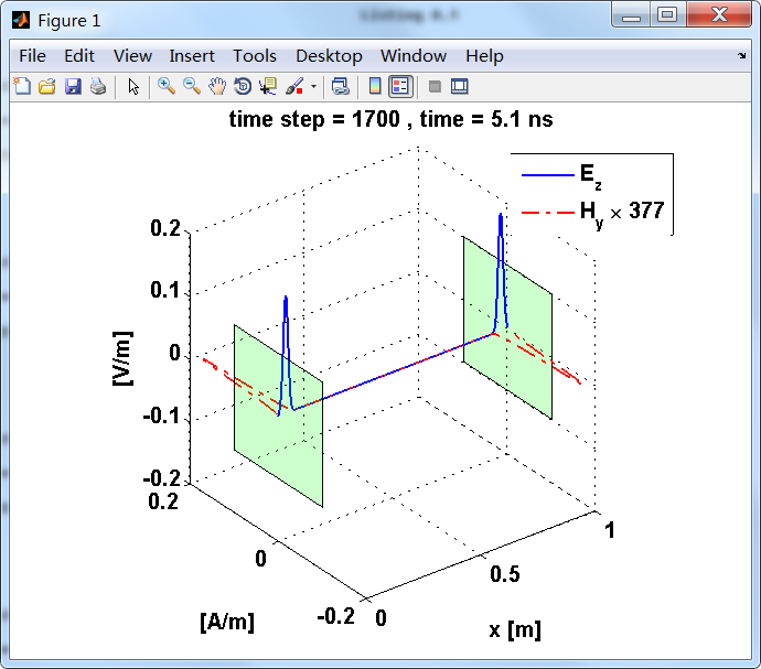
　　运行结果：

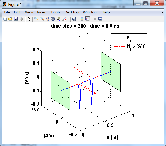
上图，从PEC板反射后，电场分量极性变反，磁场分量极性不变。

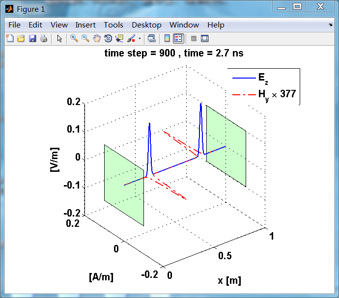
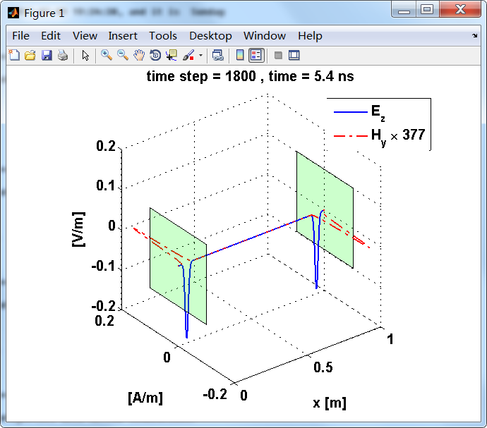
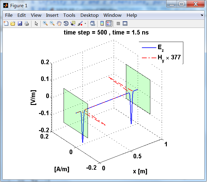
反射后，电场分量极性再次改变；