flink 实现ConnectedComponents 连通分量，增量迭代算法（Delta Iteration）实现详解

1、连通分量是什么？

首先需要了解什么是连通图、无向连通图、极大连通子图等概念，这些概念都来自数据结构-图，这里简单介绍一下。

下图是连通图和非连通图，都是无向的，这里不扩展有向图：

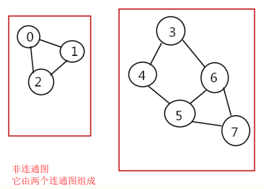
连通分量（connected component）：无向图中的极大连通子图（maximal connected subgraph）称为原图的连通分量。

极大连通子图：
1.连通图只有一个极大连通子图，就是它本身。（是唯一的）
2.非连通图有多个极大连通子图。（非连通图的极大连通子图叫做连通分量，每个分量都是一个连通图）
3.称为极大是因为如果此时加入任何一个不在图的点集中的点都会导致它不再连通。

如果需要继续了解连通图相关的内容可以自行百度。

2、flink 实现连通分量算法，本例中将分量值小的数据传递到其他连接点，通过增量迭代实现。

2.1、数据准备

public class ConnectedComponentsData {
    public static final long[] VERTICES  = new long[] {
            1, 2, 3, 4, 5, 6, 7, 8, 9, 10, 11, 12, 13, 14, 15, 16};

    public static DataSet<Long> getDefaultVertexDataSet(ExecutionEnvironment env) {
        List<Long> verticesList = new LinkedList<Long>();
        for (long vertexId : VERTICES) {
            verticesList.add(vertexId);
        }
        return env.fromCollection(verticesList);
    }

    public static final Object[][] EDGES = new Object[][] {
            new Object[]{1L, 2L},
            new Object[]{2L, 3L},
            new Object[]{2L, 4L},
            new Object[]{3L, 5L},
            new Object[]{6L, 7L},
            new Object[]{8L, 9L},
            new Object[]{8L, 10L},
            new Object[]{5L, 11L},
            new Object[]{11L, 12L},
            new Object[]{10L, 13L},
            new Object[]{9L, 14L},
            new Object[]{13L, 14L},
            new Object[]{1L, 15L},
            new Object[]{16L, 1L}
    };

    public static DataSet<Tuple2<Long, Long>> getDefaultEdgeDataSet(ExecutionEnvironment env) {

        List<Tuple2<Long, Long>> edgeList = new LinkedList<Tuple2<Long, Long>>();
        for (Object[] edge : EDGES) {
            edgeList.add(new Tuple2<Long, Long>((Long) edge[0], (Long) edge[1]));
        }
        return env.fromCollection(edgeList);
    }

}

2.2 算法实现，代码里有详细注释

/**
 * @Description:
 * 使用delta迭代实现连通分量算法。
 * 最初，算法为每个顶点分配唯一的ID。在每个步骤中，顶点选择其自身ID及其邻居ID的最小值作为其新ID，并告知其邻居其新ID。算法完成后，同一组件中的所有顶点将具有相同的ID。
 *
 * 组件ID未更改的顶点不需要在下一步中传播其信息。因此，该算法可通过delta迭代轻松表达。我们在这里将解决方案集建模为具有当前组件ID的顶点，并将工作集设置为更改的顶点。因为我们最初看到所有顶点都已更改，所以初始工作集和初始解决方案集是相同的。
 * 此外，解决方案集的增量也是下一个工作集。
 * 输入文件是纯文本文件，必须格式如下：
 *
 * 顶点表示为ID并用换行符分隔。
 * 例如，"1\n2\n12\n42\n63"给出五个顶点（1），（2），（12），（42）和（63）。
 * 边缘表示为顶点ID的对，由空格字符分隔。边线由换行符分隔。
 * 例如，"1 2\n2 12\n1 12\n42 63"给出四个（无向）边缘（1） - （2），（2） - （12），（1） - （12）和（42） - （63）。
 * 用法：ConnectedComponents --vertices <path> --edges <path> --output <path> --iterations <n>
 * 如果未提供参数，则使用{@link ConnectedComponentsData}中的默认数据和10次迭代运行程序。
 *
 **/
public class ConnectedComponents {

    //获取顶点数据
    private static DataSet<Long> getVertexDataSet(ParameterTool params, ExecutionEnvironment env){
        if(params.has("vertices")){
            return env.readCsvFile(params.get("vertices")).types(Long.class)
                    .map(new MapFunction<Tuple1<Long>, Long>() {
                        @Override
                        public Long map(Tuple1<Long> value) throws Exception {
                            return value.f0;
                        }
                    });
        }else{
            System.out.println("Executing Connected Components example with default vertices data set.");
            System.out.println("Use --vertices to specify file input.");
            return ConnectedComponentsData.getDefaultVertexDataSet(env);
        }
    }

    //获取边数据
    private static DataSet<Tuple2<Long,Long>> getEdgeDataSet(ParameterTool params,ExecutionEnvironment env){
        if(params.has("edges")){
            return env.readCsvFile(params.get("edges")).fieldDelimiter(" ").types(Long.class,Long.class);
        }else {
            System.out.println("Executing Connected Components example with default edges data set.");
            System.out.println("Use --edges to specify file input.");
            return ConnectedComponentsData.getDefaultEdgeDataSet(env);
        }
    }

    public static void main(String args[]) throws Exception{
        final ParameterTool params = ParameterTool.fromArgs(args);

        ExecutionEnvironment env = ExecutionEnvironment.getExecutionEnvironment();

        //缺省10次迭代，或者从参数中获取
        final int maxIterations = params.getInt("iterations",10);

        //make parameters available in the web interface
        env.getConfig().setGlobalJobParameters(params);

        // read vertex and edge data
        DataSet<Long> vertices = getVertexDataSet(params, env);
        //对应的加了一组反转的边
        DataSet<Tuple2<Long,Long>> edges = getEdgeDataSet(params, env).flatMap(new UndirectEdge());

        // assign the initial components (equal to the vertex id)
        //初始化顶点元组
        DataSet<Tuple2<Long, Long>> verticesWithInitialId =
                vertices.map(new DuplicateValue<>());

        // open a delta iteration
        DeltaIteration<Tuple2<Long,Long>,Tuple2<Long,Long>> iteration = verticesWithInitialId
                .iterateDelta(verticesWithInitialId,maxIterations,0);

        // apply the step logic: join with the edges, select the minimum neighbor, update if the component of the candidate is smaller
        DataSet<Tuple2<Long, Long>> changes = iteration.getWorkset().join(edges)
                .where(0).equalTo(0)
                .with(new NeighborWithComponentIDJoin())
                .groupBy(0).aggregate(Aggregations.MIN, 1)
                .join(iteration.getSolutionSet()).where(0).equalTo(0)
                .with(new ComponentIdFilter());

        // close the delta iteration (delta and new workset are identical)
        DataSet<Tuple2<Long, Long>> result = iteration.closeWith(changes, changes);

        // emit result
        if (params.has("output")) {
            result.writeAsCsv(params.get("output"), "\n", " ");
            // execute program
            env.execute("Connected Components Example");
        } else {
            System.out.println("Printing result to stdout. Use --output to specify output path.");
            result.print();
        }

    }

    /**
     * Undirected edges by emitting for each input edge the input edges itself and an inverted version.
     * 因为是无向连通图，反转边元组edges是为了将所有顶点(vertex)都放在Tuple2的第一个元素中,
     * 这样合并原来的元组和反转的元组后，生成的新元组的第一个元素将包括所有的顶点vertex，下一步就可以用join进行关联
     */
    public static final class UndirectEdge implements FlatMapFunction<Tuple2<Long,Long>,Tuple2<Long,Long>>{
        Tuple2<Long,Long> invertedEdge = new Tuple2<>();
        @Override
        public void flatMap(Tuple2<Long, Long> value, Collector<Tuple2<Long, Long>> out) throws Exception {
            invertedEdge.f0 = value.f1;
            invertedEdge.f1 = value.f0;

            out.collect(value);
            out.collect(invertedEdge);
        }
    }

    /**
     * Function that turns a value into a 2-tuple where both fields are that value.
     * 将每个点（vertex）映射成（id，id），表示用id值初始化顶点(vertex)的Component-ID （分量ID）
     * 实际上是（Vertex-ID, Component-ID）对，这个Component-ID就是需要比较以及传播的值
     */
    @FunctionAnnotation.ForwardedFields("*->f0")
    public static final class DuplicateValue<T> implements MapFunction<T,Tuple2<T,T>>{
        @Override
        public Tuple2<T, T> map(T value) throws Exception {
            return new Tuple2<>(value,value);
        }
    }

    /**
     * UDF that joins a (Vertex-ID, Component-ID) pair that represents the current component that
     * a vertex is associated with, with a (Source-Vertex-ID, Target-VertexID) edge. The function
     * produces a (Target-vertex-ID, Component-ID) pair.
     * 通过(Vertex-ID, Component-ID)顶点对与(Source-Vertex-ID, Target-VertexID)边对的连接，
     * 得到(Target-vertex-ID, Component-ID)对，这个对是相连顶点的新的分量值，
     * 下一步这个相连顶点分量值将与原来的自己的分量值比较大小，并保留小的那一对，通过增量迭代传播。
     * 这个地方有点烧脑。这个步骤主要目的就是传播分量。
     */
    @FunctionAnnotation.ForwardedFieldsFirst("f1->f1")
    @FunctionAnnotation.ForwardedFieldsSecond("f1->f0")
    public static final class NeighborWithComponentIDJoin implements JoinFunction<Tuple2<Long, Long>, Tuple2<Long, Long>, Tuple2<Long, Long>> {

        @Override
        public Tuple2<Long, Long> join(Tuple2<Long, Long> vertexWithComponent, Tuple2<Long, Long> edge) {
            return new Tuple2<>(edge.f1, vertexWithComponent.f1);
        }
    }

    /**
     * Emit the candidate (Vertex-ID, Component-ID) pair if and only if the
     * candidate component ID is less than the vertex's current component ID.
     * 从上一步的(Target-vertex-ID, Component-ID)对与SolutionSet里的原始数据进行比对，保留小的，
     * 增量迭代部分由系统框架实现了。
     */
    @FunctionAnnotation.ForwardedFieldsFirst("*")
    public static final class ComponentIdFilter implements FlatJoinFunction<Tuple2<Long, Long>, Tuple2<Long, Long>, Tuple2<Long, Long>> {

        @Override
        public void join(Tuple2<Long, Long> candidate, Tuple2<Long, Long> old, Collector<Tuple2<Long, Long>> out) {
            if (candidate.f1 < old.f1) {
                out.collect(candidate);
            }
        }
    }

}

3、执行结果

(3,1)
(7,6)
(1,1)
(11,1)
(12,1)
(6,6)
(15,1)
(5,1)
(4,1)
(16,1)
(13,8)
(9,8)
(14,8)
(2,1)
(10,8)
(8,8)