Python 数据科学系列 の Numpy、Series 和 DataFrame介绍
本課主題
- Numpy 的介绍和操作实战
- Series 的介绍和操作实战
- DataFrame 的介绍和操作实战
Numpy 的介绍和操作实战
numpy 是 Python 在数据计算领域里很常用的模块
import numpy as np

np.array([11,22,33]) #接受一个列表数据
- 创建 numpy array
>>> import numpy as np

>>> mylist = [1,2,3]

>>> x = np.array(mylist)

>>> x

array([1, 2, 3])

>>> y = np.array([4,5,6])

>>> y

array([4, 5, 6])

>>> m = np.array([[7,8,9],[10,11,12]])

>>> m

array([[ 7,  8,  9],

       [10, 11, 12]])
创建 numpy array(例子)
- 查看 numpy array 的
>>> m.shape #array([1, 2, 3])

(2, 3)

>>> x.shape #array([4, 5, 6])

(3,)

>>> y.shape #array([[ 7,  8,  9], [10, 11, 12]])

(3,) - numpy.arrange
>>> n = np.arange(0,30,2)

>>> n

array([ 0,  2,  4,  6,  8, 10, 12, 14, 16, 18, 20, 22, 24, 26, 28])
numpy.arrange( )(例子)
- 改变numpy array的位置
>>> n = np.arange(0,30,2)

>>> n

array([ 0,  2,  4,  6,  8, 10, 12, 14, 16, 18, 20, 22, 24, 26, 28])

>>> n.shape

(15,)

>>> n = n.reshape(3,5) #从15列改成3列5行

>>> n

array([[ 0,  2,  4,  6,  8],

       [10, 12, 14, 16, 18],

       [20, 22, 24, 26, 28]])
numpy.reshape( )(例子一)
>>> o = np.linspace(0,4,9)

>>> o

array([ 0. ,  0.5,  1. ,  1.5,  2. ,  2.5,  3. ,  3.5,  4. ])

>>> o.resize(3,3)

>>> o

array([[ 0. ,  0.5,  1. ],

       [ 1.5,  2. ,  2.5],

       [ 3. ,  3.5,  4. ]])
numpy.reshape( )(例子二)
- numpy.ones( ) ,numpy.zeros( ),numpy.eye( )
>>> r1 = np.ones((3,2))

>>> r1

array([[ 1.,  1.],

       [ 1.,  1.],

       [ 1.,  1.]])

>>> r1 = np.zeros((2,3))

>>> r1

array([[ 0.,  0.,  0.],

       [ 0.,  0.,  0.]])

>>> r2 = np.eye(3)

>>> r2

array([[ 1.,  0.,  0.],

       [ 0.,  1.,  0.],

       [ 0.,  0.,  1.]])
numpy.ones/zeros/eye( )(例子)
可以定义整数
>>> r5 = np.ones([2,3], int)

>>> r5

array([[1, 1, 1],

       [1, 1, 1]])

>>> r5 = np.ones([2,3])

>>> r5

array([[ 1.,  1.,  1.],

       [ 1.,  1.,  1.]])
numpy.ones(x,int)(例子)
- numpy.diag( )
>>> y = np.array([4,5,6])

>>> y

array([4, 5, 6])

>>> np.diag(y)

array([[4, 0, 0],

       [0, 5, 0],

       [0, 0, 6]])
diag( )(例子)
- 复制 numpy array
>>> r3 = np.array([1,2,3] * 3)

>>> r3

array([1, 2, 3, 1, 2, 3, 1, 2, 3])

>>> r4 = np.repeat([1,2,3],3)

>>> r4

array([1, 1, 1, 2, 2, 2, 3, 3, 3])
复制numpy array(例子)
- numpy中的 vstack和 hstack
>>> r5 = np.ones([2,3], int)

>>> r5

array([[1, 1, 1],

       [1, 1, 1]])

>>> r6 = np.vstack([r5,2*r5])

>>> r6

array([[1, 1, 1],

       [1, 1, 1],

       [2, 2, 2],

       [2, 2, 2]])

>>> r7 = np.hstack([r5,2*r5])

>>> r7

array([[1, 1, 1, 2, 2, 2],

       [1, 1, 1, 2, 2, 2]])
numpy.vstack( )和np.hstack( )(例子)
- numpy 中的加减乘除操作一 (+-*/)
>>> mylist = [1,2,3]

>>> x = np.array(mylist)

>>> y = np.array([4,5,6])

>>> x+y

array([5, 7, 9])

>>> x-y

array([-3, -3, -3])

>>> x*y

array([ 4, 10, 18])

>>> x**2

array([1, 4, 9])

>>> x.dot(y)

32
numpy中的加减乘除(例子一)
- numpy 中的加减乘除操作二:sum( )、max( )、min( )、mean( )、std( )
>>> a = np.array([1,2,3,4,5])

>>> a.sum()

15

>>> a.max()

5

>>> a.min()

1

>>> a.mean()

3.0

>>> a.std()

1.4142135623730951

>>> a.argmax()

4

>>> a.argmin()

0
numpy中的加减乘除(例子二)
- 查看numpy array 的数据类型
>>> y = np.array([4,5,6])

>>> z = np.array([y, y**2])

>>> z

array([[ 4,  5,  6],

       [16, 25, 36]])

>>> z.shape

(2, 3)

>>> z.T.shape

(3, 2)

>>> z.dtype

dtype('int64')

>>> z = z.astype('f')

>>> z.dtype

dtype('float32')
numpy array 的数据类型
- numpy 中的索引和切片
>>> s = np.arange(13)

>>> s

array([ 0,  1,  2,  3,  4,  5,  6,  7,  8,  9, 10, 11, 12])

>>> s = np.arange(13) ** 2

>>> s

array([  0,   1,   4,   9,  16,  25,  36,  49,  64,  81, 100, 121, 144])

>>> s[0],s[4],s[0:3]

(0, 16, array([0, 1, 4]))

>>> s[1:5]

array([ 1,  4,  9, 16])

>>> s[-4:]

array([ 81, 100, 121, 144])

>>> s[-5:-2]

array([ 64,  81, 100])
numpy索引和切片(例子一)
>>> r = np.arange(36)

>>> r.resize((6,6))

>>> r

array([[ 0,  1,  2,  3,  4,  5],

       [ 6,  7,  8,  9, 10, 11],

       [12, 13, 14, 15, 16, 17],

       [18, 19, 20, 21, 22, 23],

       [24, 25, 26, 27, 28, 29],

       [30, 31, 32, 33, 34, 35]])

>>> r[2,2]

14

>>> r[3,3:6]

array([21, 22, 23])

>>> r[:2,:-1]

array([[ 0,  1,  2,  3,  4],

       [ 6,  7,  8,  9, 10]])

>>> r[-1,::2]

array([30, 32, 34])

>>> r[r > 30] #取r大于30的数据

array([31, 32, 33, 34, 35])

>>> re2 = r[r > 30] = 30

>>> re2

30

>>> r8 = r[:3,:3]

>>> r8

array([[ 0,  1,  2],

       [ 6,  7,  8],

       [12, 13, 14]])

>>> r8[:] = 0

>>> r8

array([[0, 0, 0],

       [0, 0, 0],

       [0, 0, 0]])

>>> r

array([[ 0,  0,  0,  3,  4,  5],

       [ 0,  0,  0,  9, 10, 11],

       [ 0,  0,  0, 15, 16, 17],

       [18, 19, 20, 21, 22, 23],

       [24, 25, 26, 27, 28, 29],

       [30, 30, 30, 30, 30, 30]])
numpy索引和切片(例子二)
- copy numpy array 的数组
>>> r = np.arange(36)

>>> r.resize((6,6))

>>> r_copy = r.copy()

>>> r

array([[ 0,  1,  2,  3,  4,  5],

       [ 6,  7,  8,  9, 10, 11],

       [12, 13, 14, 15, 16, 17],

       [18, 19, 20, 21, 22, 23],

       [24, 25, 26, 27, 28, 29],

       [30, 31, 32, 33, 34, 35]])

>>> r_copy

array([[ 0,  1,  2,  3,  4,  5],

       [ 6,  7,  8,  9, 10, 11],

       [12, 13, 14, 15, 16, 17],

       [18, 19, 20, 21, 22, 23],

       [24, 25, 26, 27, 28, 29],

       [30, 31, 32, 33, 34, 35]])

>>> r_copy[:] = 10

>>> r_copy

array([[10, 10, 10, 10, 10, 10],

       [10, 10, 10, 10, 10, 10],

       [10, 10, 10, 10, 10, 10],

       [10, 10, 10, 10, 10, 10],

       [10, 10, 10, 10, 10, 10],

       [10, 10, 10, 10, 10, 10]])
copy( )例子
- 其他操作
>>> test = np.random.randint(0,10,(4,3))

>>> test

array([[3, 5, 2],

       [7, 7, 9],

       [8, 9, 2],

       [2, 9, 1]])

>>> for row in test:

...     print(row)

...

[3 5 2]

[7 7 9]

[8 9 2]

[2 9 1]

>>> for i in range(len(test)):

...     print(test[i])

...

[3 5 2]

[7 7 9]

[8 9 2]

[2 9 1]

>>> for i, row in enumerate(test):

...     print('row', i, 'is', row)

...

row 0 is [3 5 2]

row 1 is [7 7 9]

row 2 is [8 9 2]

row 3 is [2 9 1]

>>> test2 = test ** 2

>>> test2

array([[ 9, 25,  4],

       [49, 49, 81],

       [64, 81,  4],

       [ 4, 81,  1]])

>>> for i,j, in zip(test,test2):

...     print(i, '+', j, '=', i + j)

...

[3 5 2] + [ 9 25  4] = [12 30  6]

[7 7 9] + [49 49 81] = [56 56 90]

[8 9 2] + [64 81  4] = [72 90  6]

[2 9 1] + [ 4 81  1] = [ 6 90  2]

>>>
numpy array 的其他操作例子
Series 的介绍和操作实战
如果是输入一个字典类型的话,字典的键会自动变成 Index,然后它的值是Value
from pandas import Series, DataFrame

import pandas as pd

pd.Series(['Dog','Bear','Tiger','Moose','Giraffe','Hippopotamus','Mouse'], name='Animals') #接受一个列表类型的数据
def __init__(self, data=None, index=None, dtype=None, name=None,

                 copy=False, fastpath=False):
Series的__init__方法
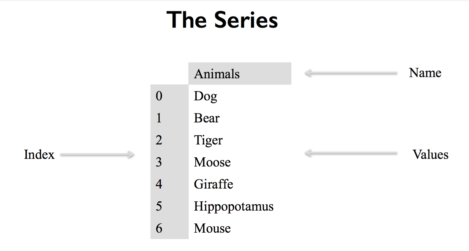
- 创建 Series 类型
第一:你可以传入一个列表或者是字典来创建 Series,如果传入的是列表,Python会自动把 [0,1,2] 作为 Series 的索引。
第二:如果你传入的是字符串类型的数据,Series 返回的dtype是object;如果你传入的是数字类型的数据,Series 返回的dtype是int64>>> from pandas import Series, DataFrame
>>> import pandas as pd
>>> animals = ['Tiger','Bear','Moose'] >>> s1 = pd.Series(animals)
>>> s1
0 Tiger
1 Bear
2 Moose
dtype: object >>> s2 = pd.Series([1,2,3])
>>> s2
0 1
1 2
2 3
dtype: int64创建 Series
Series如何处理 NaN的数据?
>>> animals2 = ['Tiger','Bear',None]

>>> s3 = pd.Series(animals2)

>>> s3

0    Tiger

1     Bear

2     None

dtype: object

>>> s4 = pd.Series([1,2,None])

>>> s4

0    1.0

1    2.0

2    NaN

dtype: float64
Series NaN数据(范例)
- Series 中的 NaN数据和如何检查 NaN数据是否相等,这时候需要调用 np.isnan( )方法
>>> import numpy as np

>>> np.nan == None

False

>>> np.nan == np.nan

False

>>> np.isnan(np.nan)

True
np.isnan( )
- Series 默应 Index 是 [0,1,2],但也可以自定义 Series 中的Index
>>> import numpy as np

>>> sports = {

...     'Archery':'Bhutan',

...     'Golf':'Scotland',

...     'Sumo':'Japan',

...     'Taekwondo':'South Korea'

... }

>>> s5 = pd.Series(sports)

>>> s5

Archery           Bhutan

Golf            Scotland

Sumo               Japan

Taekwondo    South Korea

dtype: object

>>> s5.index

Index(['Archery', 'Golf', 'Sumo', 'Taekwondo'], dtype='object')
自定义 Series 中的Index(例子一)
>>> from pandas import Series, DataFrame

>>> import pandas as pd

>>> s6 = pd.Series(['Tiger','Bear','Moose'], index=['India','America','Canada'])

>>> s6

India      Tiger

America     Bear

Canada     Moose

dtype: object
自定义 Series 中的Index(例子一)
- 查询 Series 的数据有两种方法,第一是通过index方法 e.g. s.iloc[2];第二是通过label方法 e.g. s.loc['America']
>>> from pandas import Series, DataFrame

>>> import pandas as pd

>>> s6

India      Tiger

America     Bear

Canada     Moose

dtype: object

>>> s6.iloc[2] #获取 index2位置的数据

'Moose'

>>> s6.loc['America'] #获取 label: America 的值

'Bear'

>>> s6[1] #底层调用了 s6.iloc[1]

'Bear'

>>> s6['India'] #底层调用了 s6.loc['India']

'Tiger'
查询Series(例子)
- Series 的数据操作: sum( ),它底层也是调用 numpy 的方法
>>> s7 = pd.Series([100.00,120.00,101.00,3.00])

>>> s7

0    100.0

1    120.0

2    101.0

3      3.0

dtype: float64

>>> total = 0

>>> for item in s7:

...     total +=item

...

>>> total

324.0

>>> total2 =  np.sum(s7)

>>> total2

324.0
np.sum(s7)
>>> s8 = pd.Series(np.random.randint(0,1000,10000))

>>> s8.head()

0     25

1    399

2    326

3    479

4    603

dtype: int64

>>> len(s8)

10000
head( )例子
- Series 也可以存储混合型数据
>>> s9 = pd.Series([1,2,3])

>>> s9.loc['Animals'] = 'Bears'

>>> s9

0              1

1              2

2              3

Animals    Bears

dtype: object
混合型存储数据(例子)
- Series 中的 append( ) 用法
>>> original_sports = pd.Series({'Archery':'Bhutan',

...                              'Golf':'Scotland',

...                              'Sumo':'Japan',

...                              'Taekwondo':'South Korea'})

>>> cricket_loving_countries = pd.Series(['Australia', 'Barbados','Pakistan','England'],

...                                      index=['Cricket','Cricket','Cricket','Cricket'])

>>> all_countries = original_sports.append(cricket_loving_countries)

>>> original_sports

Archery           Bhutan

Golf            Scotland

Sumo               Japan

Taekwondo    South Korea

dtype: object

>>> cricket_loving_countries

Cricket    Australia

Cricket     Barbados

Cricket     Pakistan

Cricket      England

dtype: object

>>> all_countries

Archery           Bhutan

Golf            Scotland

Sumo               Japan

Taekwondo    South Korea

Cricket        Australia

Cricket         Barbados

Cricket         Pakistan

Cricket          England

dtype: object
Series类型的append( )
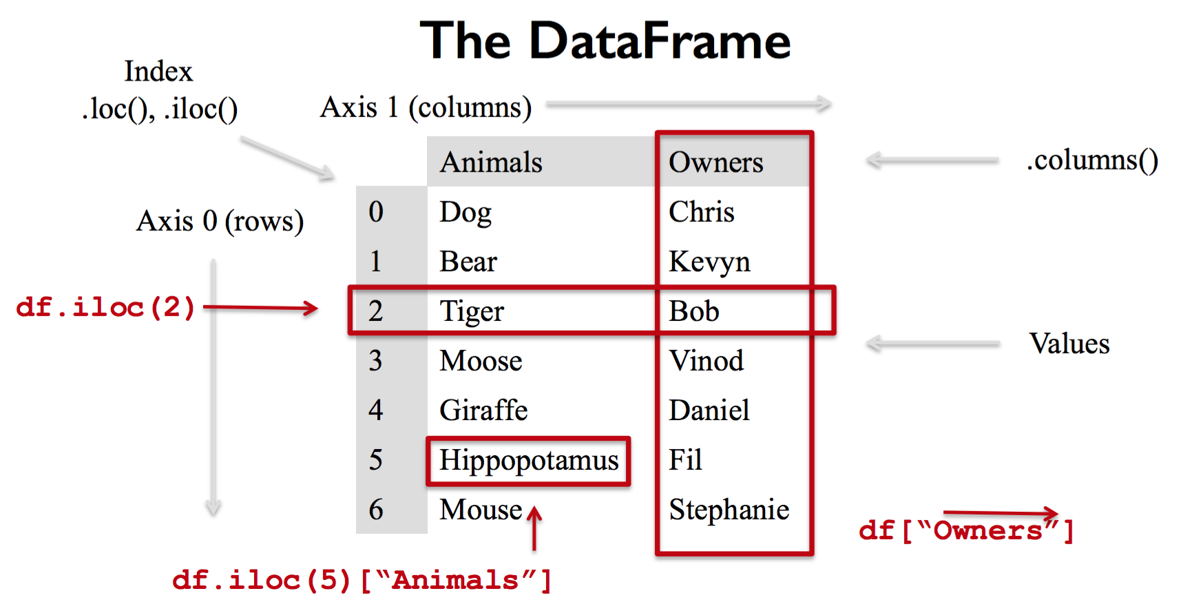
DataFrame
这是创建一个DataFrame对象的基本语句:接受字典类型的数据;字典中的Key (e.g. Animals, Owners) 对应 DataFrame中的Columns,它的 Value 也相当于数据库表中的每一行数据。
data = {

        'Animals':['Dog','Bear','Tiger','Moose','Giraffe','Hippopotamus','Mouse'],

        'Owners':['Chris','Kevyn','Bob','Vinod','Daniel','Fil','Stephanie']

}

df = DataFrame(data, columns=['Animals','Owners'])
基础操作
- 创建DataFrame
>>> from pandas import Series, DataFrame

>>> import pandas as pd

>>> data = {'name':['yahoo','google','facebook'],

...         'marks':[200,400,800],

...         'price':[9,3,7]}

>>> df = DataFrame(data)

>>> df

   marks      name  price

0    200     yahoo      9

1    400    google      3

2    800  facebook      7
创建DataFrame(例子一)
>>> df2 = DataFrame(data, columns=['name','price','marks'])

>>> df2

       name  price  marks

0     yahoo      9    200

1    google      3    400

2  facebook      7    800

>>> df3 = DataFrame(data, columns=['name','price','marks'], index=['a','b','c'])

>>> df3

       name  price  marks

a     yahoo      9    200

b    google      3    400

c  facebook      7    800

>>> df4 = DataFrame(data, columns=['name','price','marks', 'debt'], index=['a','b','c'])

>>> df4

       name  price  marks debt

a     yahoo      9    200  NaN

b    google      3    400  NaN

c  facebook      7    800  NaN
创建DataFrame(例子二)
>>> import pandas as pd

>>> purchase_1 = pd.Series({'Name':'Chris','Item Purchased':'Dog Food','Cost':22.50})

>>> purchase_2 = pd.Series({'Name':'Kelvin','Item Purchased':'Kitty Litter','Cost':2.50})

>>> purchase_3 = pd.Series({'Name':'Vinod','Item Purchased':'Bird Seed','Cost':5.00})

>>>

>>> df = pd.DataFrame([purchase_1,purchase_2,purchase_3],index=['Store 1','Store 2','Store 1'])

>>> df

         Cost Item Purchased    Name

Store 1  22.5       Dog Food   Chris

Store 2   2.5   Kitty Litter  Kelvin

Store 1   5.0      Bird Seed   Vinod
创建DataFrame(例子三)
- 查询 dataframe 的index:df.loc['index']
>>> df.loc['Store 2']

Cost                       2.5

Item Purchased    Kitty Litter

Name                    Kelvin

Name: Store 2, dtype: object
df.loc['Store 2']
>>> df.loc['Store 1']

         Cost Item Purchased   Name

Store 1  22.5       Dog Food  Chris

Store 1   5.0      Bird Seed  Vinod
df.loc['Store 1']
>>> df['Item Purchased']

Store 1        Dog Food

Store 2    Kitty Litter

Store 1       Bird Seed

Name: Item Purchased, dtype: object
df['Item Purchased']
- 查 store1 的 cost 是多少
>>> df.loc['Store 1', 'Cost']

Store 1    22.5

Store 1     5.0

Name: Cost, dtype: float64
df.loc['Store 1', 'Cost']
- 查询Cost大于3的Name
>>> df['Name'][df['Cost']>3]

Store 1    Chris

Store 1    Vinod

Name: Name, dtype: object
df['Name'][df['Cost']>3]
- 查询DataFrame 的类型
>>> type(df.loc['Store 2'])

<class 'pandas.core.series.Series'>
type( )例子
- drop dataframe (但这不会把原来的 dataframe drop 掉)
>>> df.drop('Store 1')

         Cost Item Purchased    Name

Store 2   2.5   Kitty Litter  Kelvin

>>> df

         Cost Item Purchased    Name

Store 1  22.5       Dog Food   Chris

Store 2   2.5   Kitty Litter  Kelvin

Store 1   5.0      Bird Seed   Vinod
df.drop('Store 1')
>>> copy_df = df.copy()

>>> copy_df

         Cost Item Purchased    Name

Store 1  22.5       Dog Food   Chris

Store 2   2.5   Kitty Litter  Kelvin

Store 1   5.0      Bird Seed   Vinod

>>> copy_df = df.drop('Store 1')

>>> copy_df

         Cost Item Purchased    Name

Store 2   2.5   Kitty Litter  Kelvin
把dataframe数据drop的例子
也可以用 del 把 Column 列删除掉
>>> del copy_df['Name']

>>> copy_df

         Cost Item Purchased

Store 2   2.5   Kitty Litter
del copy_df['Name']
- set_index
- rename column
- 可以修改dataframe里的数据
>>> df = pd.DataFrame([purchase_1,purchase_2,purchase_3],index=['Store 1','Store 2','Store 1'])

>>> df

         Cost Item Purchased    Name

Store 1  22.5       Dog Food   Chris

Store 2   2.5   Kitty Litter  Kelvin

Store 1   5.0      Bird Seed   Vinod

>>> df['Cost'] = df['Cost'] * 0.8

>>> df

         Cost Item Purchased    Name

Store 1  18.0       Dog Food   Chris

Store 2   2.0   Kitty Litter  Kelvin

Store 1   4.0      Bird Seed   Vinod
df['Cost'] * 0.8
>>> df = pd.DataFrame([purchase_1,purchase_2,purchase_3],index=['Store 1','Store 2','Store 1'])

>>> costs = df['Cost']

>>> costs

Store 1    22.5

Store 2     2.5

Store 1     5.0

Name: Cost, dtype: float64

>>> costs += 2

>>> costs

Store 1    24.5

Store 2     4.5

Store 1     7.0

Name: Cost, dtype: float64
costs = df['Cost']
进阶操作
- Merge
Full Outer Join
Inner Join
Left Join
Right Join - apply
- group by
- agg
- astype
- cut
s = pd.Series([168, 180, 174, 190, 170, 185, 179, 181, 175, 169, 182, 177, 180, 171])

pd.cut(s, 3)

pd.cut(s, 3, labels=['Small', 'Medium', 'Large'])
cut( )
- pivot table
Date in DataFrame
- Timestampe
- period
- DatetimeINdex
- PeriodIndex
- to_datetime
- Timedelta
- date_range
- difference between date value
- resample
- asfreq - changing the frequency of the date
读取 csv 文件
import pandas as pd

pd.read_csv('student.csv')
- 读取csv
>>> from pandas import Series, DataFrame

>>> import pandas as pd

>>> df_student = pd.read_csv('student.csv')

>>> df_student

        name   class  marks  age

    janice  python     80   22

      alex  python     95   21

     peter  python     85   25

       ken    java     75   28

 lawerance    java     50   22
pd.read_csv('student.csv')(例子一)
df_student = pd.read_csv('student.csv', index_col=0, skiprows=1)pd.read_csv('student.csv')(例子二)
- 获取分数大于70的数据
>>> df_student['marks'] > 70

    True

    True

    True

    True

   False

Name: marks, dtype: bool
方法一: df_student['marks'] > 70
>>> df_student.where(df_student['marks']>70)

     name   class  marks   age

 janice  python   80.0  22.0

   alex  python   95.0  21.0

  peter  python   85.0  25.0

    ken    java   75.0  28.0

    NaN     NaN    NaN   NaN
方法二: df_student.where(df_student['marks']>70)
>>> df_student[df_student['marks'] > 70]

     name   class  marks  age

0  janice  python     80   22

1    alex  python     95   21

2   peter  python     85   25

3     ken    java     75   28
方法三: df_student[df_student['marks'] > 70]
- 获取class = 'python' 的数据,df.count( ) 是不会把 NaN数据计算在其中
>>> df2 = df_student.where(df_student['class'] == 'python')

>>> df2

     name   class  marks   age

0  janice  python   80.0  22.0

1    alex  python   95.0  21.0

2   peter  python   85.0  25.0

3     NaN     NaN    NaN   NaN

4     NaN     NaN    NaN   NaN

>>> df2 = df_student[df_student['class'] == 'python']

>>> df2

     name   class  marks  age

0  janice  python     80   22

1    alex  python     95   21

2   peter  python     85   25
df_student.where( )例子
- 计算 class 的数目 e.g. count( )
>>> df2['class'].count() #不会把 NaN也计算

3

>>> df_student['class'].count() #会把 NaN也计算

5
df.count( )例子
- 删取NaN数据
>>> df3 = df2.dropna()

>>> df3

     name   class  marks   age

0  janice  python   80.0  22.0

1    alex  python   95.0  21.0

2   peter  python   85.0  25.0
df2.dropna()
- 获取age大于23 学生的数据
>>> df_student

        name   class  marks  age

0     janice  python     80   22

1       alex  python     95   21

2      peter  python     85   25

3        ken    java     75   28

4  lawerance    java     50   22

>>> df_student[df_student['age'] > 23]

    name   class  marks  age

2  peter  python     85   25

3    ken    java     75   28

>>> df_student['age'] > 23

0    False

1    False

2     True

3     True

4    False

Name: age, dtype: bool

>>> len(df_student[df_student['age'] > 23])

2
df_student[df_student['age'] > 23]
- 获取age大于23和分数大于80分学生的数据
>>> df_student

        name   class  marks  age

0     janice  python     80   22

1       alex  python     95   21

2      peter  python     85   25

3        ken    java     75   28

4  lawerance    java     50   22

>>> df_and = df_student[(df_student['age'] > 23) & (df_student['marks'] > 80)]

>>> df_and

    name   class  marks  age

2  peter  python     85   25
df_student[(df_student['age'] > 23) & (df_student['marks'] > 80)]
- 获取age大于23或分数大于80分学生的数据
>>> df_student

        name   class  marks  age

0     janice  python     80   22

1       alex  python     95   21

2      peter  python     85   25

3        ken    java     75   28

4  lawerance    java     50   22

>>> df_or = df_student[(df_student['age'] > 23) | (df_student['marks'] > 80)]

>>> df_or

    name   class  marks  age

1   alex  python     95   21

2  peter  python     85   25

3    ken    java     75   28
df_student[(df_student['age'] > 23) | (df_student['marks'] > 80)]
- 重新定义index的数值 df.set_index( )
>>> df_student = pd.read_csv('student.csv')

>>> df_student

        name   class  marks  age

0     janice  python     80   22

1       alex  python     95   21

2      peter  python     85   25

3        ken    java     75   28

4  lawerance    java     50   22

>>> df_student['order_id'] = df_student.index

>>> df_student

        name   class  marks  age  order_id

0     janice  python     80   22         0

1       alex  python     95   21         1

2      peter  python     85   25         2

3        ken    java     75   28         3

4  lawerance    java     50   22         4

>>> df_student = df_student.set_index('class')

>>> df_student

             name  marks  age  order_id

class

python     janice     80   22         0

python       alex     95   21         1

python      peter     85   25         2

java          ken     75   28         3

java    lawerance     50   22         4
df_student.set_index( )例子
- 获取在 dataframe column 中唯一的数据
>>> df_student = pd.read_csv('student.csv')

>>> df_student['class'].unique()

array(['python', 'java'], dtype=object)
df.unique( )例子
python 的可视化 matplotlib
- plot
參考資料
Coursera: Introduction to Data Science in Python
Data Science: GoodHart's Law | Goodhart's Law
Python 数据科学系列 の Numpy、Series 和 DataFrame介绍的更多相关文章
- Python数据科学手册-Numpy入门
通过Python有效导入.存储和操作内存数据的技巧 数据来源:文档.图像.声音.数值等等,将所有的数据简单的看做数字数组 非常有助于 理解和处理数据 不管数据是何种形式,第一步都是 将这些数据转换成 ...
- [python]-数据科学库Numpy学习
一.Numpy简介: Python中用列表(list)保存一组值,可以用来当作数组使用,不过由于列表的元素可以是任何对象,因此列表中所保存的是对象的指针.这样为了保存一个简单的[1,2,3],需要有3 ...
- Python数据科学手册-Numpy的结构化数组
结构化数组 和 记录数组 为复合的.异构的数据提供了非常有效的存储 (一般使用pandas 的 DataFrame来实现) 传入的dtpye 使用 Numpy数据类型 Character Descri ...
- Python数据科学手册-Numpy数组的排序
1) Numpy中的快速排序: np.sort 和 np.argsort np.sort 是快速排序,算法复杂度 O[ N log N] ,也可以选择归并排序和堆排序 如果不想修改原始输入数组,返 ...
- Python数据科学手册-Numpy数组的计算:比较、掩码和布尔逻辑,花哨的索引
Numpy的通用函数可以用来替代循环, 快速实现数组的逐元素的 运算 同样,使用其他通用函数实现数组的逐元素的 比较 < > 这些运算结果 是一个布尔数据类型的数组. 有6种标准的比较操作 ...
- Python数据科学手册-Numpy数组的计算,通用函数
Python的默认实现(CPython)处理某些操作非常慢,因为动态性和解释性, CPython 在每次循环必须左数据类型的检查和函数的调度..在编译是进行这样的操作.就会加快执行速度. 通用函数介绍 ...
- Python数据科学手册-Numpy数组的计算:广播
广播可以简单理解为用于不同大小数组的二元通用函数(加减乘等)的一组规则 二元运算符是对相应元素逐个计算 广播允许这些二元运算符可以用于不同大小的数组 更高维度的数组 更复杂的情况,对俩个数组的同时广播 ...
- python书籍推荐:Python数据科学手册
所属网站分类: 资源下载 > python电子书 作者:today 链接:http://www.pythonheidong.com/blog/article/448/ 来源:python黑洞网 ...
- 干货!小白入门Python数据科学全教程
前言 本文讲解了从零开始学习Python数据科学的全过程,涵盖各种工具和方法 你将会学习到如何使用python做基本的数据分析 你还可以了解机器学习算法的原理和使用 说明 先说一段题外话.我是一名数据 ...
随机推荐
- Linux下批量修改文件名方法
对于在Linux中修改文件名的方式一般我们会用mv命令进行修改,但是mv命令是无法处理大量文件修改名称. 但是在处理大量文件的时候该如何进行批量修改呢? 方法一:mv配合for循环方式进行修改 [ro ...
- Cocos2d-x 3.0 Android改动APK名、更改图标、改动屏幕方向、改动版本,一些须要注意的问题
非常多新手程序员做出一个游戏后,编译成apk安装在手机上.却发现安装程序名和游戏图标都是Cocos2dx默认的,并且默认屏幕方向是横向.那么须要怎么才干改动为自己想要的呢? 打开你创建的project ...
- Object-C与Swift混合开发
Object-C作为Apple的iOS App开发语言服务了很多个年头,2014年Apple推出了新的编程语言Swift.更高效更安全的口号再次吸引了一大批非iOS开发程序猿进入,小编觉得Swift代 ...
- swift手记-4
// // ViewController.swift // learn4 // // Created by myhaspl on 16/1/23. // Copyright (c) 2016年 myh ...
- 入门vue----(vue的安装)
1.安装node.js 2.基于node.js,利用淘宝npm镜像安装相关依赖 在cmd里直接输入:npm install -g cnpm –registry=https://registry.npm ...
- JS排序
冒泡排序 https://sort.hust.cc/1.bubbleSort.html 选择排序 https://sort.hust.cc/2.selectionSort.html 插入排序 http ...
- path和classpath细节
从学习java的最初我们就被要求先设置path变量和classpath变量.但是这两个环境变量到底有什么作用呢? 1.path环境变量 path环境变量的主要作用是告诉操作系统到哪里去寻找某个程序,如 ...
- Java加密与解密笔记(三) 非对称加密
非对称的特点是加密和解密时使用的是不同的钥匙.密钥分为公钥和私钥,用公钥加密的数据只能用私钥进行解密,反之亦然. 另外,密钥还可以用于数字签名.数字签名跟上文说的消息摘要是一个道理,通过一定方法对数据 ...
- ERROR: Java 1.7 or later is required to run Apache Drill.
问题 Apache 的 drill 执行启动命令 drill-embedded 报错: ERROR: Java 1.7 or later is required to run Apache Drill ...
- iOS cocos2d游戏引擎的了解之一
ios游戏引擎之Cocos2d(一) cocos2d是一个免费开源的ios游戏开发引擎,并且完全采用object-c进行编写,这对于已经用惯object-c进行ios应用开发的童鞋来说非常容易上手.这 ...