标签传播算法(llgc 或 lgc)

动手实践标签传播算法

复现论文：Learning with Local and Global Consistency^[1]

lgc 算法可以参考：DecodePaper/notebook/lgc

初始化算法

载入一些必备的库：

from IPython.display import set_matplotlib_formats
%matplotlib inline
#set_matplotlib_formats('svg', 'pdf')

import numpy as np
import matplotlib.pyplot as plt
from scipy.spatial.distance import cdist
from sklearn.datasets import make_moons

save_dir = '../data/images'

创建一个简单的数据集

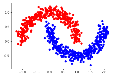
利用 make_moons 生成一个半月形数据集。

n = 800   # 样本数
n_labeled = 10 # 有标签样本数
X, Y = make_moons(n, shuffle=True, noise=0.1, random_state=1000)

X.shape, Y.shape

((800, 2), (800,))

def one_hot(Y, n_classes):
    '''
    对标签做 one_hot 编码

    参数
    =====
    Y: 从 0 开始的标签
    n_classes: 类别数
    '''
    out = Y[:, None] == np.arange(n_classes)
    return out.astype(float)

color = ['red' if l == 0 else 'blue' for l in Y]
plt.scatter(X[:, 0], X[:, 1], color=color)
plt.savefig(f"{save_dir}/bi_classification.pdf", format='pdf')
plt.show()

Y_input = np.concatenate((one_hot(Y[:n_labeled], 2), np.zeros((n-n_labeled, 2))))

算法过程：

Step 1: 创建相似度矩阵 W

def rbf(x, sigma):
    return np.exp((-x)/(2* sigma**2))

sigma = 0.2
dm = cdist(X, X, 'euclidean')
W = rbf(dm, sigma)
np.fill_diagonal(W, 0)   # 对角线全为 0

Step 2: 计算 S

\[S = D^{-\frac{1}{2}} W D^{-\frac{1}{2}}
\]

向量化编程：

def calculate_S(W):
    d = np.sum(W, axis=1)
    D_ = np.sqrt(d*d[:, np.newaxis]) # D_ 是 np.sqrt(np.dot(diag(D),diag(D)^T))
    return np.divide(W, D_, where=D_ != 0)

S = calculate_S(W)

迭代一次的结果

alpha = 0.99
F = np.dot(S, Y_input)*alpha + (1-alpha)*Y_input

Y_result = np.zeros_like(F)
Y_result[np.arange(len(F)), F.argmax(1)] = 1

Y_v = [1 if x == 0 else 0 for x in Y_result[0:,0]]

color = ['red' if l == 0 else 'blue' for l in Y_v]
plt.scatter(X[0:,0], X[0:,1], color=color)
#plt.savefig("iter_1.pdf", format='pdf')
plt.show()

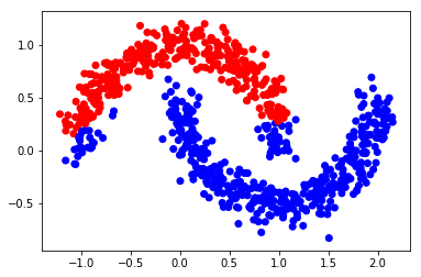
Step 3: 迭代 F "n_iter" 次直到收敛

n_iter = 150
F = Y_input
for t in range(n_iter):
    F = np.dot(S, F)*alpha + (1-alpha)*Y_input

Step 4: 画出最终结果

Y_result = np.zeros_like(F)
Y_result[np.arange(len(F)), F.argmax(1)] = 1

Y_v = [1 if x == 0 else 0 for x in Y_result[0:,0]]

color = ['red' if l == 0 else 'blue' for l in Y_v]
plt.scatter(X[0:,0], X[0:,1], color=color)
#plt.savefig("iter_n.pdf", format='pdf')
plt.show()

from sklearn import metrics

print(metrics.classification_report(Y, F.argmax(1)))

acc = metrics.accuracy_score(Y, F.argmax(1))
print('准确度为',acc)

              precision    recall  f1-score   support

           0       1.00      0.86      0.92       400
           1       0.88      1.00      0.93       400

   micro avg       0.93      0.93      0.93       800
   macro avg       0.94      0.93      0.93       800
weighted avg       0.94      0.93      0.93       800

准确度为 0.92875

sklearn 实现 lgc

参考：https://scikit-learn.org/stable/modules/label_propagation.html

在 sklearn 里提供了两个 lgc 模型：LabelPropagation 和 LabelSpreading，其中后者是前者的正则化形式。\(W\) 的计算方式提供了 rbf 与 knn。

• rbf 核由参数 gamma控制（\(\gamma=\frac{1}{2{\sigma}^2}\)）
• knn 核 由参数 n_neighbors（近邻数）控制

def pred_lgc(X, Y, F, numLabels):
    from sklearn import preprocessing
    from sklearn.semi_supervised import LabelSpreading
    cls = LabelSpreading(max_iter=150, kernel='rbf', gamma=0.003, alpha=.99)
    # X.astype(float) 为了防止报错 "Numerical issues were encountered "
    cls.fit(preprocessing.scale(X.astype(float)), F)
    ind_unlabeled = np.arange(numLabels, len(X))
    y_pred = cls.transduction_[ind_unlabeled]
    y_true = Y[numLabels:].astype(y_pred.dtype)
    return y_true, y_pred

Y_input = np.concatenate((Y[:n_labeled], -np.ones(n-n_labeled)))
y_true, y_pred = pred_lgc(X, Y, Y_input, n_labeled)
print(metrics.classification_report(Y, F.argmax(1)))

              precision    recall  f1-score   support

           0       1.00      0.86      0.92       400
           1       0.88      1.00      0.93       400

   micro avg       0.93      0.93      0.93       800
   macro avg       0.94      0.93      0.93       800
weighted avg       0.94      0.93      0.93       800

networkx 实现 lgc

参考：networkx.algorithms.node_classification.lgc.local_and_global_consistency 具体的细节，我还没有研究！先放一个简单的例子：

G = nx.path_graph(4)
G.node[0]['label'] = 'A'
G.node[3]['label'] = 'B'
G.nodes(data=True)

G.edges()

predicted = node_classification.local_and_global_consistency(G)
predicted

['A', 'A', 'B', 'B']

更多精彩内容见：DecodePaper 觉得有用，记得给个 star !(@DecodePaper)

---

1. Zhou D, Bousquet O, Lal T N, et al. Learning with Local and Global Consistency[C]. neural information processing systems, 2003: 321-328. ↩︎