MATLAB 图像打开保存

一、图片读取保存

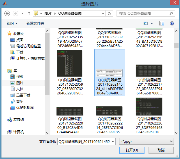
（1）读取

clear all
[filename,pathname]=uigetfile({'*.jpg';'*.bmp';'*.gif'},'选择图片');
if isequal(filename,0)
    disp('Users Selected Canceled');
else
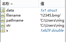
str=[pathname filename];
im = imread(str);
imshow(im);
end

（2）保存

clear all
x=0:0.01:2*pi;
plot(x,sin(x));

[filename,pathname]=uiputfile({'*.bmp';},'保存图片');%路径和图片名
if ~isequal(filename,0)
    str = [pathname filename];%路径名
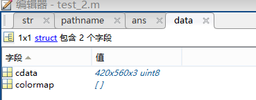
    data= getframe(gcf);%图片内容数据
    imwrite(data.cdata,str,'bmp');
%     saveas(gcf,str,'bmp');%两种方式都可以保存图片
    close(gcf);
 else
    disp('保存失败');
end

二、灰度图和彩色图

(1)

图像中的单个点称为像素(pixel)，每个像素都有一个值，称为像素值，它表示特定颜色的强度。

对于黑白图，是指每个像素的颜色用二进制的1位来表示，那末颜色只有“1”和“0”这两个值。这也就是说，要么是黑，要么是白。

对于灰度图，如果不用合成的方式来表达，可以表示为（0），（123），（255）。

如果用颜色合成的方式来表达，即它的一个像素值往往用R，G，B三个分量表示，注意，是RGB合成来表示一个像素的颜色。但要注意的                    是RGB  分量必须都相等，否则就成彩色了。比如为（0，0，0）为黑，（123，123，123）为某种灰色，（255，255，255）为白。

clear all;
[filename,pathname]=uigetfile('*.*','select an image');
sample=imread([pathname filename]);%原始图
gray=rgb2gray(sample);%灰白图
bw=im2bw(sample);%黑白图
subplot(311),imshow(sample);
title('原图')
subplot(312),imshow(gray);
title('灰度图')
subplot(313),imshow(bw);
title('黑白图')

　

（2）rgb三分量分别表示

r=sample(:,:,1);
g=sample(:,:,2);
b=sample(:,:,3);
subplot(131),imshow(r);
subplot(132),imshow(g);
subplot(133),imshow(b);

　　

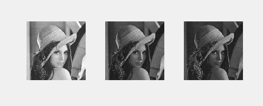
三、filter2、conv2和imfilter 平滑处理

（1）

clear all;
clear all
[filename,pathname]=uigetfile('*.*','select an image');
sample=imread([pathname filename]);

mean3Sample = filter2(fspecial('average',3),sample)/255;
mean5Sample = filter2(fspecial('average',5),sample)/255;
mean7Sample = filter2(fspecial('average',7),sample)/255;
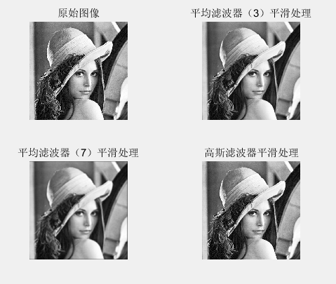
gaussianSample = filter2(fspecial('gaussian'),sample)/255;

subplot(2,2,1);
imshow(sample); %原始图像
title('原始图像')

subplot(2,2,2);
imshow(mean3Sample); %采用均值进行平滑处理
title('平均滤波器（3）平滑处理')

subplot(2,2,3);
imshow(mean7Sample); %原始图像
title('平均滤波器（7）平滑处理')

subplot(2,2,4);
imshow(gaussianSample); %高斯滤波器进行平滑处理
title('高斯滤波器平滑处理')

conv3Sample = conv2(fspecial('average',3),sample)/255;
conv7Sample = conv2(fspecial('average',7),sample)/255;
convSample = conv2(fspecial('gaussian'),sample)/255;

figure
subplot(321),imshow(mean3Sample)
title('filter2滤波')
subplot(322),imshow(conv3Sample)
title('conv2法')

subplot(323),imshow(mean7Sample)
subplot(324),imshow(conv7Sample)

subplot(325),imshow(gaussianSample)
subplot(326),imshow(convSample)

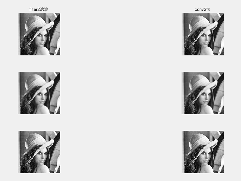
这两个函数只能针对二维图像。滤波器本质就是加权。

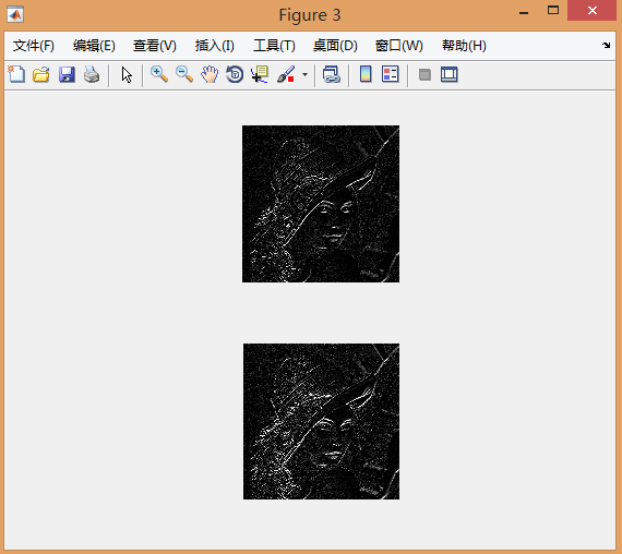
（2）分别采用’prewitt’和’sobel’边缘算子对图像做边缘增强处理，并显示边缘处理后的图像

figure
%采用’prewitt’算子:
prewittSample = uint8(filter2(fspecial('prewitt'),sample));
subplot(211),imshow(prewittSample);
%采用’ sobel’算子:
sobelSample = uint8(filter2(fspecial('sobel'),sample));
subplot(212),imshow(sobelSample);

　

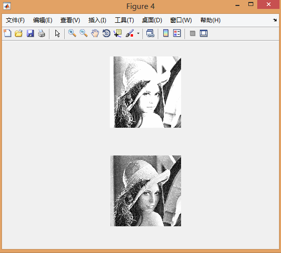
(3)采用“原图*2-平滑图像”，以及“原图+边缘处理图像”的方法锐化图像

figure
%采用“原图*2-平滑图像”方法:
subSample = sample.*2 - uint8(mean7Sample);
subplot(211),imshow(subSample);
%采用“原图+边缘处理图像”方法
addSample = sample + uint8(prewittSample);
subplot(212),imshow(addSample);

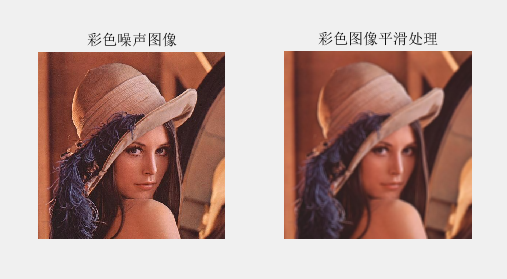
(4)imfilter 彩色图像的平滑

clear all;
I = imread('lena.jpg');      %读取一张噪声图像
%提取图像的三个（R、G、B）分量图像
R = I(:,:,1);
G = I(:,:,2);
B = I(:,:,3);
%生成一个8x8的均值滤波器
w = fspecial('average',8);
fR = imfilter(R,w,'replicate');
fG = imfilter(G,w,'replicate');
fB = imfilter(B,w,'replicate');
fc_filtered = cat(3,fR,fG,fB);   %三分量平滑后合为一个整体
figure
subplot(121); imshow(I);title('彩色噪声图像');
subplot(122); imshow(fc_filtered);title('彩色图像平滑处理'); 

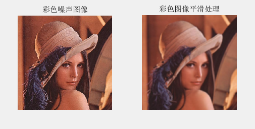
clear all;
I = imread('lena.jpg');      %读取一张噪声图像
%提取图像的三个（R、G、B）分量图像
R = I(:,:,1);
G = I(:,:,2);
B = I(:,:,3);
%生成一个8x8的均值滤波器
w = fspecial('average',8);
fc_filtered = imfilter(I, w, 'replicate'); %不用rgb分量单独平滑，彩色图像的平滑函数
figure
subplot(121); imshow(I);title('彩色噪声图像');2
subplot(122); imshow(fc_filtered);title('彩色图像平滑处理');

四、锐化处理

锐化本质是边缘增强，可以采用原图加边缘增强得到

（1）

clear all
A=imread('123.png');
figure(1);
subplot(2,2,1);
imshow(A);
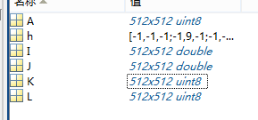
title('原图');

I=double(A);
h=[-1 -1 -1;-1 9 -1;-1 -1 -1];
J=conv2(I,h,'same');
K=uint8(J);
subplot(2,2,2);
imshow(J);
title('使用拉普拉斯算子锐化处理后的图(double格式)');
subplot(2,2,3);
imshow(K);
title('使用拉普拉斯算子锐化处理后的图(uint8格式)');
L=(K+A)/2;
subplot(2,2,4);
imshow(L);
title('原图+锐化');

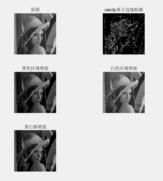
（2）

clear all
A=imread('123.png');
figure(1);
subplot(3,2,1);
imshow(A);
title('原图');

BW=edge(A,'canny');%黑白图
subplot(3,2,2);
imshow(BW);
title('candy算子边缘检测');

K=uint8(BW);%转换格式，1白色
M=uint8(~K);%反转数值，1黑色
L_1=A-50*M;%黑色区域增强
subplot(3,2,3);
imshow(L_1);
title('黑色区域增强');
L_2=(A+K*50);%白色区域增强
subplot(3,2,4);
imshow(L_2);
title('白色区域增强');

L_3=A-50*M+50*K;
subplot(3,2,5);
imshow(L_3);
title('黑白都增强');

（3）

clear all;
I=imread('lena.jpg');
subplot(3,2,1),imshow(I);
xlabel('a)原始图像');

H=fspecial('sobel');%sobel滤波器
J=imfilter(I, H, 'replicate');%灰度值
subplot(3,2,3),imshow(J);
xlabel('Sobel锐化滤波处理');
K=I+0.32*J;%比例相加
subplot(324),imshow(K)
xlabel('Sobel锐化滤波处理+原图');

H=fspecial('laplacian');%laplacian滤波器
J=imfilter(I, H, 'replicate');%灰度值
subplot(3,2,5),imshow(J);
xlabel('laplacian锐化滤波处理');
K=I+J;%比例相加
subplot(326),imshow(K)
xlabel('laplacian锐化滤波处理+原图');

滤波器决定了是锐化或者平滑

五、RGB和HSI

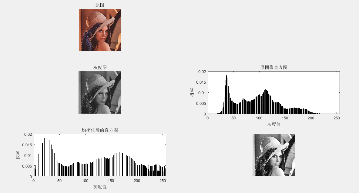
（1）直方图均衡

clear all
sourcePic=imread('lena.jpg');
[m,n,o]=size(sourcePic);
grayPic=rgb2gray(sourcePic);%灰度图
subplot(321),imshow(sourcePic); title('原图')
subplot(323),imshow(grayPic); title('灰度图')

gp=zeros(1,256); %计算各灰度出现的概率 （0,255）出现的概率
for i=1:256
    gp(i)=length(find(grayPic==(i-1)))/(m*n); %i灰度的概率
end
subplot(324),,bar(0:255,gp);
title('原图像直方图');
xlabel('灰度值');
ylabel('概率');
axis([0 256 0 0.02])  

newGp=zeros(1,256); %计算新的各灰度出现的概率
S1=zeros(1,256);
S2=zeros(1,256);
tmp=0;
for i=1:256
    tmp=tmp+gp(i);
    S1(i)=tmp;  %累计概率（映射到0~1）
    S2(i)=round(S1(i)*256); %映射到0~255
end
%映射
for i=1:256
    newGp(i)=sum(gp(find(S2==(i-1)))); %灰度值为联系
end
subplot(325),bar(0:255,newGp);
title('均衡化后的直方图');
xlabel('灰度值');
ylabel('概率');
axis([0 256 0 0.02])  

newGrayPic=grayPic; %填充各像素点新的灰度值
for i=1:256
    newGrayPic(find(grayPic==(i-1)))=S2(i);
end
subplot(326),imshow(newGrayPic);

clear all
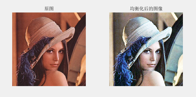
sourcePic=imread('lena.jpg');
[m,n,o]=size(sourcePic);
subplot(121),imshow(sourcePic);
title('原图')
%%
grayPic=sourcePic(:,:,1);
gp=zeros(1,256); %计算各灰度出现的概率
for i=1:256
    gp(i)=length(find(grayPic==(i-1)))/(m*n);
end  

newGp=zeros(1,256); %计算新的各灰度出现的概率
S1=zeros(1,256);
S2=zeros(1,256);
tmp=0;
for i=1:256
    tmp=tmp+gp(i);
    S1(i)=tmp;
    S2(i)=round(S1(i)*256);
end
for i=1:256
    newGp(i)=sum(gp(find(S2==i)));
end  

newGrayPic=grayPic; %填充各像素点新的灰度值
for i=1:256
    newGrayPic(find(grayPic==(i-1)))=S2(i);
end
nr=newGrayPic;
 %%
grayPic=sourcePic(:,:,2);  

gp=zeros(1,256); %计算各灰度出现的概率
for i=1:256
    gp(i)=length(find(grayPic==(i-1)))/(m*n);
end  

newGp=zeros(1,256); %计算新的各灰度出现的概率
S1=zeros(1,256);
S2=zeros(1,256);
tmp=0;
for i=1:256
    tmp=tmp+gp(i);
    S1(i)=tmp;
    S2(i)=round(S1(i)*256);
end
for i=1:256
    newGp(i)=sum(gp(find(S2==i)));
end  

newGrayPic=grayPic; %填充各像素点新的灰度值
for i=1:256
    newGrayPic(find(grayPic==(i-1)))=S2(i);
end
ng=newGrayPic;
%%
grayPic=sourcePic(:,:,3);  

gp=zeros(1,256); %计算各灰度出现的概率
for i=1:256
    gp(i)=length(find(grayPic==(i-1)))/(m*n);
end  

newGp=zeros(1,256); %计算新的各灰度出现的概率
S1=zeros(1,256);
S2=zeros(1,256);
tmp=0;
for i=1:256
    tmp=tmp+gp(i);
    S1(i)=tmp;
    S2(i)=round(S1(i)*256);
end
for i=1:256
    newGp(i)=sum(gp(find(S2==i)));
end  

newGrayPic=grayPic; %填充各像素点新的灰度值
for i=1:256
    newGrayPic(find(grayPic==(i-1)))=S2(i);
end
nb=newGrayPic;
%%
res=cat(3,nr,ng,nb);
subplot(122),imshow(res);
title('均衡化后的图像')

(2)hsi(色调、饱和度、亮度)和hsv（色调（H），饱和度（S），明度（V））。

clear all
% hsi = rgb2hsi(rgb)把一幅RGB图像转换为HSI图像，
% 输入图像是一个彩色像素的M×N×3的数组，
% 其中每一个彩色像素都在特定空间位置的彩色图像中对应红、绿、蓝三个分量。
% 假如所有的RGB分量是均衡的，那么HSI转换就是未定义的。
% 输入图像可能是double（取值范围是[0, 1]），uint8或 uint16。
%
% 输出HSI图像是double，
% 其中hsi(:, :, 1)是色度分量，它的范围是除以2*pi后的[0, 1]；
% hsi(:, :, 2)是饱和度分量，范围是[0, 1]；
% hsi(:, :, 3)是亮度分量，范围是[0, 1]。

% 抽取图像分量
rgb=imread('lena.jpg');
rgb = im2double(rgb);
r = rgb(:, :, 1);
g = rgb(:, :, 2);
b = rgb(:, :, 3);

% 执行转换方程
num = 0.5*((r - g) + (r - b));
den = sqrt((r - g).^2 + (r - b).*(g - b));
theta = acos(num./(den + eps)); %防止除数为0

H = theta;
H(b > g) = 2*pi - H(b > g);
H = H/(2*pi);

num = min(min(r, g), b);
den = r + g + b;
den(den == 0) = eps; %防止除数为0

S = 1 - 3.* num./den;
H(S == 0) = 0;
I = (r + g + b)/3;

% 将3个分量联合成为一个HSI图像
hsi = cat(3, H, S, I);
subplot(121),imshow(hsi)
title('hsi图像')

subplot(122),imshow(rgb2hsv(rgb))%自带函数
title('hsv图形')