Java 使用 Apache commons-math3 线性拟合、非线性拟合实例（带效果图）

Java 使用 CommonsMath3 的线性和非线性拟合实例，带效果图

例子查看

• GitHub
• Gitee
• 运行src/main/java/org/wfw/chart/Main.java 即可查看效果
• src/main/java/org/wfw/math 包下是简单的使用

版本说明

• JDK:1.8
• commons-math:3.6.1

一些基础知识

• 线性：两个变量之间存在一次方函数关系，就称它们之间存在线性关系。也就是如下的函数：

\[f(x)=kx+b
\]

• 非线性：除了线性其他的都是非线性，例如：

\[f(x)=e^x
\]

• 矩阵：矩阵（Matrix）是一个按照长方阵列排列的复数或实数集合，可以理解为平面或者空间的坐标点。
  
  看大佬怎么说之>> B站-线性代数的本质 - 系列合集

• 微分、积分：互为逆过程，一句话概括，微分就是求导，求某个点的极小变化量的斜率。积分是求一些列变化点的和，几何意义是面积
  
  看大佬怎么说之>> B站-微积分的本质 - 系列合集

• 拟合：形象的说，拟合就是把平面上一系列的点，用一条光滑的曲线连接起来的过程。找到一条最符合这些散点的曲线，使得尽可能多的落在曲线上。常用的方法是最小二乘法。也就是最小二乘问题

---

添加依赖

Maven 中添加依赖

<!-- https://mvnrepository.com/artifact/org.apache.commons/commons-math3 -->
<dependency>
    <groupId>org.apache.commons</groupId>
    <artifactId>commons-math3</artifactId>
    <version>3.6.1</version>
</dependency>

如果你是 Gradle

// https://mvnrepository.com/artifact/org.apache.commons/commons-math3
compile group: 'org.apache.commons', name: 'commons-math3', version: '3.6.1'

---

如何使用和验证

1. 假设函数已知
2. 根据函数并添加随机数R生成一系列散点数据（蓝色）
3. 进行拟合，根据拟合结果生成拟合曲线
4. 对比结果曲线（绿色）和散点曲线

例如：

\[f(x) = 2x + 3
\]

首先根绝函数生成 \(x\) 取任意实数时的以及所对应的 \(f(x)\) 得到数据集 \(xy\)

\[f(x,y) = (0,3)*R, (1,5)*R, (2,7)*R...(n,2n+3)*R
\]

然后对这组数据进行拟合，然后和已知函数 \(f(x)\) 对比斜率 \(k\) 以及截距 \(b\)

---

1. 线性拟合

线性函数：

\[f(x) = kx + b
\]

假设函数为：

\[f(x) = 1.5x + 0.5
\]

生成数据集合:

/**
 *
 * y = kx + b
 * f(x) = 1.5x + 0.5
 *
 * @return
 */
public static double[][] linearScatters() {
    List<double[]> data = new ArrayList<>();
    for (double x = 0; x <= 10; x += 0.1) {
        double y = 1.5 * x + 0.5;
        y += Math.random() * 4 - 2; // 随机数
        double[] xy = {x, y};
        data.add(xy);
    }
    return data.stream().toArray(double[][]::new);
}

进行拟合

public static Result linearFit(double[][] data) {
    List<double[]> fitData = new ArrayList<>();
    SimpleRegression regression = new SimpleRegression();
    regression.addData(data); // 数据集
	/*
	 * RegressionResults 中是拟合的结果
	 * 其中重要的几个参数如下：
	 *   parameters:
	 *      0: b
	 *      1: k
	 *   globalFitInfo
	 *      0: 平方误差之和, SSE
	 *      1: 平方和, SST
	 *      2: R 平方, RSQ
	 *      3: 均方误差, MSE
	 *      4: 调整后的 R 平方, adjRSQ
	 *
	 * */
    RegressionResults results = regression.regress();
    double b = results.getParameterEstimate(0);
    double k = results.getParameterEstimate(1);
    double r2 = results.getRSquared();

    // 重新计算生成拟合曲线
    for (double[] datum : data) {
        double[] xy = {datum[0], k * datum[0] + b};
        fitData.add(xy);
    }

    StringBuilder func = new StringBuilder();
    func.append("f(x) =");
    func.append(b >= 0 ? " " : " - ");
    func.append(Math.abs(b));
    func.append(k > 0 ? " + " : " - ");
    func.append(Math.abs(k));
    func.append("x");

    return new Result(fitData.stream().toArray(double[][]::new), func.toString());
}

拟合效果

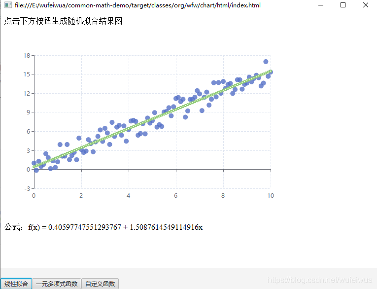
线性拟合比较简单，主要是 SimpleRegression 类的 regress() 方法，默认使用 最小二乘法优化器

---

2. 非线性（曲线）拟合（一元多项式）

非线性函数

\[f(x) = a + bx + cx^2 + dx^3 +...+ mx^n
\]

假设函数为

\[f(x) = 1 + 2x + 3x^2
\]

生成数据集合:

/**
*
* f(x) = 1 + 2x + 3x^2
*
* @return
*/
public static double[][] curveScatters() {
	List<double[]> data = new ArrayList<>();
	for (double x = 0; x <= 20; x += 1) {
	    double y = 1 + 2 * x + 3 * x * x;
	    y += Math.random() * 60 - 10; // 随机数
	    double[] xy = {x, y};
	    data.add(xy);
	}
	return data.stream().toArray(double[][]::new);
}

进行拟合

public static Result curveFit(double[][] data) {
   ParametricUnivariateFunction function = new PolynomialFunction.Parametric();/*多项式函数*/
   double[] guess = {1, 2, 3}; /*猜测值 依次为 常数项、1次项、二次项*/

   // 初始化拟合
   SimpleCurveFitter curveFitter = SimpleCurveFitter.create(function,guess);

   // 添加数据点
   WeightedObservedPoints observedPoints = new WeightedObservedPoints();
   for (double[] point : data) {
       observedPoints.add(point[0], point[1]);
   }
   /*
    * best 为拟合结果
    * 依次为 常数项、1次项、二次项
    * 对应 y = a + bx + cx^2 中的 a, b, c
    * */
   double[] best = curveFitter.fit(observedPoints.toList());

   /*
   * 根据拟合结果重新计算
   * */
   List<double[]> fitData = new ArrayList<>();
   for (double[] datum : data) {
       double x = datum[0];
       double y = best[0] + best[1] * x + best[2] * x * x; // y = a + bx + cx^2
       double[] xy = {x, y};
       fitData.add(xy);
   }

   StringBuilder func = new StringBuilder();
   func.append("f(x) =");
   func.append(best[0] > 0 ? " " : " - ");
   func.append(Math.abs(best[0]));
   func.append(best[1] > 0 ? " + " : " - ");
   func.append(Math.abs(best[1]));
   func.append("x");
   func.append(best[2] > 0 ? " + " : " - ");
   func.append(Math.abs(best[2]));
   func.append("x^2");

   return new Result(fitData.stream().toArray(double[][]::new), func.toString());
}

拟合效果

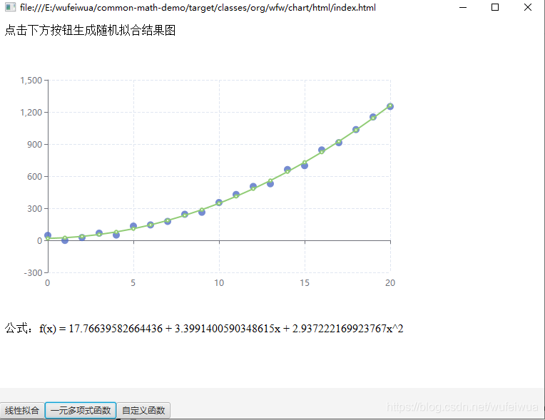
一元多项式曲线的拟合多了一些步骤。但是总归也是不难的。主要是 SimpleCurveFitter 类以及 ParametricUnivariateFunction 接口。

3. 自定义函数拟合（一元多项式）

总得来说，貌似线性和一元多项式都不难。不过，实际工作或者学术中，一般都是自定义的函数。

假设有一元多项式函数:

\[f(x) = d + \frac{a-d}{1 + (\frac{x}{c})^b}
\]

需要拟合出 a,b,c,d 四个参数的值。

方法:

1. 实现 ParametricUnivariateFunction 接口
2. 自定义函数,实现 value 方法
3. 解偏微分方程，实现 gradient 方法
4. 设置需要拟合的点
5. 调用SimpleCurveFitter#fit 方法进行拟合

不着急写代码，先看ParametricUnivariateFunction 这个接口的源码:

/**
 * An interface representing a real function that depends on one independent
 * variable plus some extra parameters.
 *
 * @since 3.0
 */
public interface ParametricUnivariateFunction {
    /**
     * Compute the value of the function.
     * 计算函数的值
     * @param x Point for which the function value should be computed.
     * @param parameters Function parameters.
     * @return the value.
     */
    double value(double x, double ... parameters);

    /**
     * Compute the gradient of the function with respect to its parameters.
     * 计算函数相对于某个参数的导数
     * @param x Point for which the function value should be computed.
     * @param parameters Function parameters.
     * @return the value.
     */
    double[] gradient(double x, double ... parameters);
}

• value 方法很简单，就是说计算函数 \(F(x)\) 的值。说人话就是自定义函数的
• gradient 方法为返回一个数组,其实意思就是求偏微分方程，对每一个要拟合的参数求导就行

不会偏微分方程？ 点这里

按格式输入你的方程=>输入自变量=>输入求导阶数(一般都是 1 阶)=>计算

好了开始写代码吧，假设函数如下：

\[f(x) = d + \frac{a-d}{1 + (\frac{x}{c})^b}
\]

1. 自定义 MyFunction 实现 ParametricUnivariateFunction 接口：

static class MyFunction implements ParametricUnivariateFunction {
	public double value(double x, double ... parameters) {
		double a = parameters[0];
		double b = parameters[1];
		double c = parameters[2];
		double d = parameters[3];
		return d + ((a - d) / (1 + Math.pow(x / c, b)));
	}

	public double[] gradient(double x, double ... parameters) {
		double a = parameters[0];
		double b = parameters[1];
		double c = parameters[2];
		double d = parameters[3];

		double[] gradients = new double[4];
		double den = 1 + Math.pow(x / c, b);

		gradients[0] = 1 / den; // 对 a 求导

		gradients[1] = -((a - d) * Math.pow(x / c, b) * Math.log(x / c)) / (den * den); // 对 b 求导

		gradients[2] = (b * Math.pow(x / c, b - 1) * (x / (c * c)) * (a - d)) / (den * den); // 对 c 求导

		gradients[3] = 1 - (1 / den); // 对 d 求导

		return gradients;

	}
}

生成数据散点

/**
*
* <pre>
*     f(x) = d + ((a - d) / (1 + Math.pow(x / c, b)))
*     a = 1500
*     b = 0.95
*     c = 65
*     d = 35000
* </pre>
*
* @return
*/
public static double[][] customizeFuncScatters() {
    MyFunction function = new MyFunction();
    List<double[]> data = new ArrayList<>();
    for (double x = 7; x <= 10000; x *= 1.5) {
        double y = function.value(x, 1500, 0.95, 65, 35000);
        y += Math.random() * 5000 - 2000; // 随机数
        double[] xy = {x, y};
        data.add(xy);
    }
    return data.stream().toArray(double[][]::new);
}

拟合自定义函数

public static Result customizeFuncFit(double[][] scatters) {
    ParametricUnivariateFunction function = new MyFunction();/*多项式函数*/
    double[] guess = {1500, 0.95, 65, 35000}; /*猜测值 依次为 a b c d 。必须和 gradient 方法返回数组对应。如果不知道都设置为 1*/

    // 初始化拟合
    SimpleCurveFitter curveFitter = SimpleCurveFitter.create(function,guess);

    // 添加数据点
    WeightedObservedPoints observedPoints = new WeightedObservedPoints();
    for (double[] point : scatters) {
        observedPoints.add(point[0], point[1]);
    }

   /*
    * best 为拟合结果 对应 a b c d
    * 可能会出现无法拟合的情况
    * 需要合理设置初始值
    * */
    double[] best = curveFitter.fit(observedPoints.toList());
    double a = best[0];
    double b = best[1];
    double c = best[2];
    double d = best[3];

    // 根据拟合结果生成拟合曲线散点
    List<double[]> fitData = new ArrayList<>();
    for (double[] datum : scatters) {
        double x = datum[0];
        double y = function.value(x, a, b, c, d);
        double[] xy = {x, y};
        fitData.add(xy);
    }

    // f(x) = d + ((a - d) / (1 + Math.pow(x / c, b)))
    StringBuilder func = new StringBuilder();
    func.append("f(x) =");
    func.append(d > 0 ? " " : " - ");
    func.append(Math.abs(d));
    func.append(" ((");
    func.append(a > 0 ? "" : "-");
    func.append(Math.abs(a));
    func.append(d > 0 ? " - " : " + ");
    func.append(Math.abs(d));
    func.append(" / (1 + ");
    func.append("(x / ");
    func.append(c > 0 ? "" : " - ");
    func.append(Math.abs(c));
    func.append(") ^ ");
    func.append(b > 0 ? " " : " - ");
    func.append(Math.abs(b));

    return new Result(fitData.stream().toArray(double[][]::new), func.toString());
}

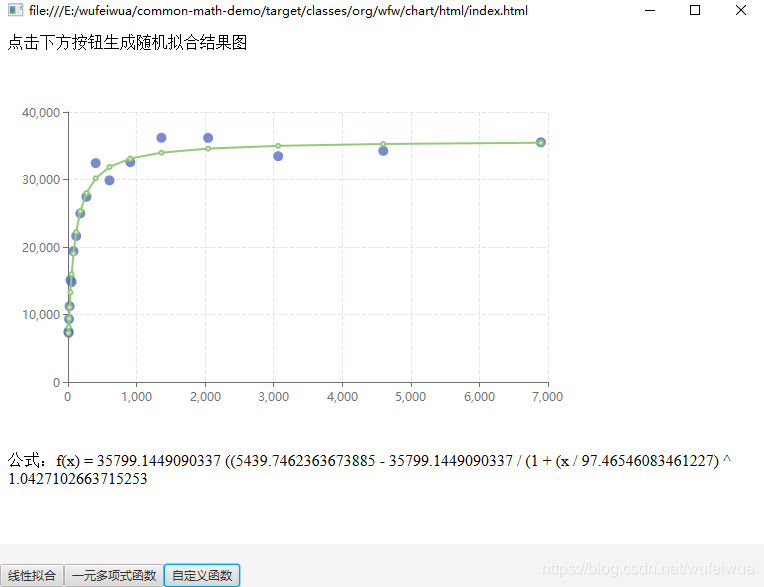
拟合效果

4. 多元多项式拟合

我用的 javafx8 版本不支持 WebGL 所以无法通过按钮直接直观展示拟合效果。我用拟合前得数据和拟合后重新计算的数据进行对比

** 方程 **

\[f(x_1,x_2) = y = a + b * x_1 + c * sin(x_2)
\]

4.1 构造数据

假设: \(a = 20, b = 2, c = 12\) ，则函数 \(f\) 为 \(f(x_1,x_2) = y = 20 + 2 * x_1 + 12 * sin(x_2)\)

根据这个函数构造数据

/**
     * 生成随机数
     */
public static double[][] randomX() {
    List<double[]> data = new ArrayList<>();
    for (double i = 0; i < 10; i += 0.1) {
        double x1 = Math.cos(i);
        double x2 = Math.sin(i);
        data.add(new double[]{x1, x2});
    }
    return data.stream().toArray(double[][]::new);
}

/**
     * f(x1,x2) = y = a + b * x1 + c * sin(x2)
     * @param arr
     * @return
     */
public static double[] randomY(double[][] arr) {
    if (arr != null && arr.length > 0) {
        int len = arr.length;
        double[] y = new double[len];
        for (int i = 0; i < len; i++) {
            // f(x1,x2) = y = 20 + x1 + 12 * sin(x2)
            double[] x = arr[i];
            // 构造数据
            y[i] = functionConstructorY(x);
        }
        return y;
    }
    return null;
}

/**
     * 已知的函数为: f(x1,x2) = y = 20 + 2 * x1 + 12 * sin(x2)
     * 即：f(x1,x2) = y = a + b * x1 + c * sin(x2) 中
     * a = 20, b = 2, c = 12
     * @param x
     * @return
     */
public static double functionConstructorY(double[] x) {
    double x1 = x[0], x2 = x[1];
    return 20 + 2 * x1 + Math.sin(10 * x2);
}

4.2 拟合

多元多项式的拟合主要用到 MultipleLinearRegression 接口，它有三个实现方式。我们选择最小二乘法的实现 OLSMultipleLinearRegression

/**
 * 多元多项式数据
 * 已知： f(x1,x2) = y = a + b * x1 + c * sin(x2)
 *
 */
public static double[][] multiVarPolyScatters() {
    double[][] x = randomX();
    double[] y = randomY(x);
    OLSMultipleLinearRegression ols = new OLSMultipleLinearRegression();
    ols.newSampleData(y, x);
    // ct 拟合的常数项（系数）。对应 a,b,c
    double[] ct = ols.estimateRegressionParameters();
}

4.3 验证

根据上面的拟合结果重新计算 \(f(x_1,x_2)\) 的值

/**
* f(x1,x2) = y = a + b * x1 + c * sin(x2)
* @param ct 拟合的常数项（系数）。对应 a,b,c
* @param x x 的值。对应 x1,x2
* @return
*/
public static double functionValueY(double[] ct, double[] x) {
    double a = ct[0], b = ct[1], c = ct[2];
    double x1 = x[0], x2 = x[1];
    return a + b * x1 + Math.sin(c * x2);
}

/**
* 多元多项式数据
* 已知： f(x1,x2) = y = a + b * x1 + c * sin(x2)
* @return
* arr[0] 对应所有的 y 的值
* arr[1] 对应所有的 x1 的值
* arr[2] 对应所有的 x2 的值
*/
public static double[][] multiVarPolyScatters() {
    double[][] x = randomX();
    double[] y = randomY(x);
    OLSMultipleLinearRegression ols = new OLSMultipleLinearRegression();
    ols.newSampleData(y, x);
    // ct 即为拟合结果
    double[] ct = ols.estimateRegressionParameters();

    double[] valueY = new double[x.length];
    for (int i = 0; i < x.length; i++) {
        // 重新计算 y 的值。与原有构造的 y 对比
        valueY[i] = functionValueY(ct, x[i]);
    }

    // 散点数据用于 Echarts 画图
    double[][] data = new double[x.length][3];// x1, x2, y
    for (int i = 0; i < valueY.length; i++) {
    	// ==================== x1 ====== x2 ======= y ====
    	data[i] = new double[]{x[i][0], x[i][1], valueY[i]};
    }
    return data;
}

4.4 画图

Echarts 3D画图的工具在 https://echarts.apache.org/examples/zh/editor.html?c=line3d-orthographic&gl=1 这个地方。我们将构造数据的函数改为我们的

// ...
var data = [];
// Parametric curve
for (var t = 0; t < 10; t += 0.1) {
    // 这里改成我们的函数。其他的都不变
    var x =  Math.cos(t);
    var y =  Math.sin(t);
    var z = 20 + 2 * x + 12 * Math.sin(y);
    data.push([x, y, z]);
}
// ...

那可以得到这样一张图

然后我们运行 org.wfw.chart.data.MultipleLinearRegressionData#main() 方法后将得到的数据整个赋值给 data 覆盖也行。我们就得到了如下的图

拟合的结果是 $$ a = 20.01068756847646, b = 2.036022472817587, c = 10.571979017911016 $$ 和我们一开始的确定好的值也差不多

4.5 多说两句

• calculateRSquared() 计算 \(R^2\)
• calculateAdjustedRSquared() 计算 \(ajdRSQ\) ，调整后的 \(R^2\)
• estimateRegressionParameters() 拟合常数项

关于 newSampleData() 方法参数的 y 和 x 样本

/**
     * Loads model x and y sample data, overriding any previous sample.
     *
     * Computes and caches QR decomposition of the X matrix.
     * @param y the [n,1] array representing the y sample
     * @param x the [n,k] array representing the x sample
     * @throws MathIllegalArgumentException if the x and y array data are not
     *             compatible for the regression
     */
    public void newSampleData(double[] y, double[][] x) throws MathIllegalArgumentException {
        validateSampleData(x, y);
        newYSampleData(y);
        newXSampleData(x);
    }

源码是这样的，y 就是 \(f(x_1,x_2)\) 的值，而 x 中的 k 代表的是 \(x_1,x_2\)​ 的值，是顺序对应的