Convolutional Neural Network-week2编程题1（Keras tutorial - 笑脸识别）

本次我们将：

• 学习到一个高级的神经网络的框架，能够运行在包括TensorFlow和CNTK的几个较低级别的框架之上的框架。
  
  看看如何在几个小时内建立一个深入的学习算法。
• 为什么我们要使用Keras框架呢？Keras是为了使深度学习工程师能够很快地建立和实验不同的模型的框架，正如TensorFlow是一个比Python更高级的框架，Keras是一个更高层次的框架，并提供了额外的抽象方法。最关键的是Keras能够以最短的时间让想法变为现实。

import numpy as np
from keras import layers
from keras.layers import Input, Dense, Activation, ZeroPadding2D, BatchNormalization, Flatten, Conv2D
from keras.layers import AveragePooling2D, MaxPooling2D, Dropout, GlobalMaxPooling2D, GlobalAveragePooling2D
from keras.models import Model
from keras.preprocessing import image
from keras.utils import layer_utils
from keras.utils.data_utils import get_file
from keras.applications.imagenet_utils import preprocess_input
import pydot
from IPython.display import SVG
from keras.utils.vis_utils import model_to_dot
from keras.utils import plot_model
from kt_utils import *

import keras.backend as K
K.set_image_data_format('channels_last')
import matplotlib.pyplot as plt
from matplotlib.pyplot import imshow

%matplotlib inline

注意：正如你所看到的，我们已经从Keras中导入了很多功能， 只需直接调用它们即可轻松使用它们。 比如：X = Input(…) 或者X = ZeroPadding2D(…).

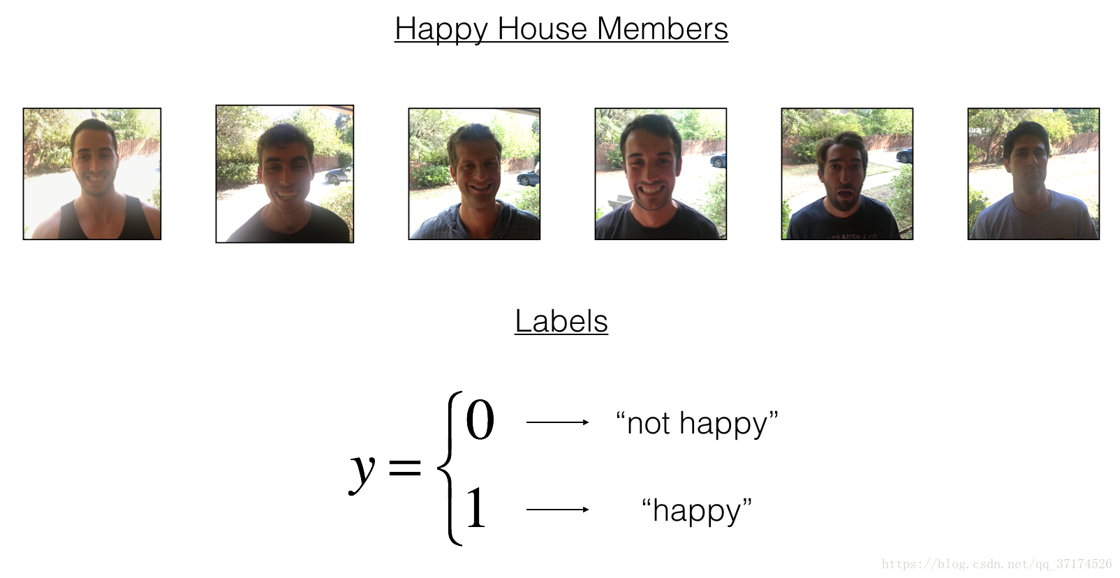
1. 任务描述

建立一个算法，它使用来自前门摄像头的图片来检查这个人是否快乐，只有在人高兴的时候，门才会打开。

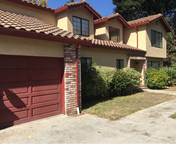
你收集了你的朋友和你自己的照片，被前门的摄像头拍了下来。数据集已经标记好了

X_train_orig, Y_train_orig, X_test_orig, Y_test_orig, classes = load_dataset()

# Normalize image vectors
X_train = X_train_orig/255.
X_test = X_test_orig/255.

# Reshape
Y_train = Y_train_orig.T
Y_test = Y_test_orig.T

print ("number of training examples = " + str(X_train.shape[0]))
print ("number of test examples = " + str(X_test.shape[0]))
print ("X_train shape: " + str(X_train.shape))
print ("Y_train shape: " + str(Y_train.shape))
print ("X_test shape: " + str(X_test.shape))
print ("Y_test shape: " + str(Y_test.shape))

number of training examples = 600

number of test examples = 150

X_train shape: (600, 64, 64, 3)

Y_train shape: (600, 1)

X_test shape: (150, 64, 64, 3)

Y_test shape: (150, 1)

Details of the "Happy" dataset:

• Images are of shape (64,64,3)

• Training: 600 pictures

• Test: 150 pictures

2. Building a model in Keras

Keras非常适合快速制作模型，它可以在很短的时间内建立一个很优秀的模型.

Here is an example of a model in Keras:

def model(input_shape):
    # Define the input placeholder as a tensor with shape input_shape. Think of this as your input image!
    X_input = Input(input_shape)

    # Zero-Padding: pads the border of X_input with zeroes
    X = ZeroPadding2D((3, 3))(X_input)

    # CONV -> BN -> RELU Block applied to X
    X = Conv2D(32, (7, 7), strides = (1, 1), name = 'conv0')(X)
    X = BatchNormalization(axis = 3, name = 'bn0')(X)
    X = Activation('relu')(X)

    # MAXPOOL
    X = MaxPooling2D((2, 2), name='max_pool')(X)

    # FLATTEN X (means convert it to a vector) + FULLYCONNECTED
    X = Flatten()(X)
    X = Dense(1, activation='sigmoid', name='fc')(X)

    # Create model. This creates your Keras model instance, you'll use this instance to train/test the model.
    model = Model(inputs = X_input, outputs = X, name='HappyModel')

    return model

注意：

• Keras框架使用的变量名和我们以前使用的numpy和TensorFlow变量不一样。它不是在前向传播的每一步上创建新变量（比如X, Z1, A1, Z2, A2,…）以便于不同层之间的计算。

• 在Keras中，我们使用X覆盖了所有的值，没有保存每一层结果，我们只需要最新的值，唯一例外的就是X_input，我们将它分离出来是因为它是输入的数据，我们要在最后的创建模型那一步中用到。

# GRADED FUNCTION: HappyModel

def HappyModel(input_shape):
    """
    Implementation of the HappyModel.

    Arguments:
    input_shape -- shape of the images of the dataset

    Returns:
    model -- a Model() instance in Keras
    """

    ### START CODE HERE ###
    # Feel free to use the suggested outline in the text above to get started, and run through the whole
    # exercise (including the later portions of this notebook) once. The come back also try out other
    # network architectures as well.
    X_input = Input(input_shape)

    # 使用0填充: X_input周围填充0, p=3
    X = ZeroPadding2D((3, 3))(X_input)

    # 使用CONV -> Batch归一化 -> Relu
    X = Conv2D(32, (3, 3), strides = (1, 1), name = 'conv0')(X)
    X = BatchNormalization(axis=3, name='bn0')(X)
    X = Activation('relu')(X)
    # MaxPool: 最大值池化层
    X = MaxPooling2D((2, 2), name='max_pool')(X)

    X = Conv2D(16, (3, 3), strides = (1, 1), name = 'conv1')(X)  # 优化后
    X = Activation('relu')(X)
    X = MaxPooling2D((2, 2), name='max_pool1')(X)

    # Flatten层, 矩阵-->向量
    # 全连接层(full Connected)
    X = Flatten()(X)
    X = Dense(1, activation='sigmoid', name='fc')(X)

    model = Model(inputs = X_input, outputs = X, name='HappyModel')

    ### END CODE HERE ###

    return model

设计好模型，训练并测试模型需要：

1. 创建一个模型实体。

2. 编译模型，可以使用这个语句：model.compile(optimizer = "...", loss = "...", metrics = ["accuracy"])。

3. 训练模型：model.fit(x = ..., y = ..., epochs = ..., batch_size = ...)。

4. 评估模型：model.evaluate(x = ..., y = ...)。

# step 1. create the model.
happyModel = HappyModel(X_train.shape[1:])

# step 2. compile the model to configure the learning process. accuracy是评价指标
happyModel.compile(optimizer = 'adam', loss = 'binary_crossentropy', metrics = ['accuracy'])

# step 3. 训练模型
happyModel.fit(x = X_train, y = Y_train, epochs = 40, batch_size = 50)

# step 4. 评价模型， 在测试集上评价
preds = happyModel.evaluate(x = X_test, y = Y_test)
print()
print ("Loss = " + str(preds[0]))
print ("Test Accuracy = " + str(preds[1]))

Epoch 1/40
600/600 [==============================] - 20s - loss: 0.7217 - acc: 0.6300
Epoch 2/40
600/600 [==============================] - 21s - loss: 0.4625 - acc: 0.8083
Epoch 3/40
600/600 [==============================] - 19s - loss: 0.3341 - acc: 0.8667
Epoch 4/40
600/600 [==============================] - 24s - loss: 0.2439 - acc: 0.9167
Epoch 5/40
600/600 [==============================] - 22s - loss: 0.1956 - acc: 0.9367
Epoch 6/40
600/600 [==============================] - 21s - loss: 0.1750 - acc: 0.9350
Epoch 7/40
600/600 [==============================] - 20s - loss: 0.1411 - acc: 0.9600
Epoch 8/40
600/600 [==============================] - 29s - loss: 0.1271 - acc: 0.9583
Epoch 9/40
600/600 [==============================] - 33s - loss: 0.1177 - acc: 0.9667
Epoch 10/40
600/600 [==============================] - 29s - loss: 0.0918 - acc: 0.9767
Epoch 11/40
600/600 [==============================] - 30s - loss: 0.0772 - acc: 0.9833
Epoch 12/40
600/600 [==============================] - 23s - loss: 0.0734 - acc: 0.9817
Epoch 13/40
600/600 [==============================] - 20s - loss: 0.0716 - acc: 0.9867
Epoch 14/40
600/600 [==============================] - 20s - loss: 0.0724 - acc: 0.9800
Epoch 15/40
600/600 [==============================] - 19s - loss: 0.0598 - acc: 0.9867
Epoch 16/40
600/600 [==============================] - 20s - loss: 0.0667 - acc: 0.9833
Epoch 17/40
600/600 [==============================] - 19s - loss: 0.0566 - acc: 0.9850
Epoch 18/40
600/600 [==============================] - 22s - loss: 0.0449 - acc: 0.9917
Epoch 19/40
600/600 [==============================] - 21s - loss: 0.0475 - acc: 0.9917
Epoch 20/40
600/600 [==============================] - 21s - loss: 0.0533 - acc: 0.9850
Epoch 21/40
600/600 [==============================] - 21s - loss: 0.0468 - acc: 0.9883
Epoch 22/40
600/600 [==============================] - 20s - loss: 0.0391 - acc: 0.9933
Epoch 23/40
600/600 [==============================] - 19s - loss: 0.0367 - acc: 0.9917
Epoch 24/40
600/600 [==============================] - 20s - loss: 0.0339 - acc: 0.9900
Epoch 25/40
600/600 [==============================] - 21s - loss: 0.0436 - acc: 0.9883
Epoch 26/40
600/600 [==============================] - 20s - loss: 0.0314 - acc: 0.9900
Epoch 27/40
600/600 [==============================] - 21s - loss: 0.0295 - acc: 0.9900
Epoch 28/40
600/600 [==============================] - 21s - loss: 0.0295 - acc: 0.9933
Epoch 29/40
600/600 [==============================] - 20s - loss: 0.0261 - acc: 0.9917
Epoch 30/40
600/600 [==============================] - 21s - loss: 0.0286 - acc: 0.9933
Epoch 31/40
600/600 [==============================] - 22s - loss: 0.0237 - acc: 0.9933
Epoch 32/40
600/600 [==============================] - 23s - loss: 0.0192 - acc: 0.9983
Epoch 33/40
600/600 [==============================] - 22s - loss: 0.0218 - acc: 0.9967
Epoch 34/40
600/600 [==============================] - 21s - loss: 0.0272 - acc: 0.9950
Epoch 35/40
600/600 [==============================] - 19s - loss: 0.0188 - acc: 0.9983
Epoch 36/40
600/600 [==============================] - 19s - loss: 0.0166 - acc: 0.9933
Epoch 37/40
600/600 [==============================] - 19s - loss: 0.0193 - acc: 0.9983
Epoch 38/40
600/600 [==============================] - 19s - loss: 0.0134 - acc: 0.9967
Epoch 39/40
600/600 [==============================] - 20s - loss: 0.0147 - acc: 0.9983
Epoch 40/40
600/600 [==============================] - 19s - loss: 0.0174 - acc: 0.9983
<keras.callbacks.History at 0x1cc49470>

150/150 [==============================] - 1s     

Loss = 0.10337299724419911
Test Accuracy = 0.9733333309491475

准确度大于80%就算正常，如果你的准确度没有大于80%，你可以尝试改变模型：

X = Conv2D(32, (3, 3), strides = (1, 1), name = 'conv0')(X)
X = BatchNormalization(axis = 3, name = 'bn0')(X)
X = Activation('relu')(X)

直到 height and width dimensions 十分小， channels数 十分大(≈32 for example)

• 你可以在每个块后面使用最大值池化层，它将会减少宽、高的维度。
• Change your optimizer. 这里使用的是Adam
• 如果模型难以运行，并且遇到了内存不够的问题，那么就降低batch_size (12通常是一个很好的折中方案)
• Run on more epochs, until you see the train accuracy plateauing.

Note: If you perform hyperparameter tuning on your model, the test set actually becomes a dev set, and your model might end up overfitting to the test (dev) set. But just for the purpose of this assignment, we won't worry about that here.

3. 总结

模型构建过程，Create -> Compile -> Fit/Train -> Evaluate/Test.

4. 测试你的图片

### START CODE HERE ###
img_path = 'images/smail01.png'
### END CODE HERE ###
img = image.load_img(img_path, target_size=(64, 64))
imshow(img)

x = image.img_to_array(img)
x = np.expand_dims(x, axis=0)
x = preprocess_input(x)

print(happyModel.predict(x))

[[1.]]

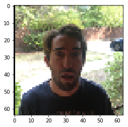
### START CODE HERE ###
img_path = 'images/smail08.png'
### END CODE HERE ###
img = image.load_img(img_path, target_size=(64, 64))
imshow(img)

x = image.img_to_array(img)
x = np.expand_dims(x, axis=0)
x = preprocess_input(x)

print(happyModel.predict(x))

[[0.]]

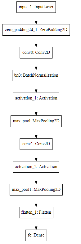
5. 其他一些有用的功能

• model.summary()：打印出你的每一层的大小细节

• plot_model() : 绘制出布局图

happyModel.summary()

______________________________________________________________
Layer (type)                 Output Shape              Param #
=================================================================
input_3 (InputLayer)         (None, 64, 64, 3)         0
_________________________________________________________________
zero_padding2d_3 (ZeroPaddin (None, 70, 70, 3)         0
_________________________________________________________________
conv0 (Conv2D)               (None, 68, 68, 32)        896
_________________________________________________________________
bn0 (BatchNormalization)     (None, 68, 68, 32)        128
_________________________________________________________________
activation_3 (Activation)    (None, 68, 68, 32)        0
_________________________________________________________________
max_pool (MaxPooling2D)      (None, 34, 34, 32)        0
_________________________________________________________________
flatten_3 (Flatten)          (None, 36992)             0
_________________________________________________________________
fc (Dense)                   (None, 1)                 36993
=================================================================
Total params: 38,017
Trainable params: 37,953
Non-trainable params: 64
_________________________________________________________________

执行下面：

需要安装:Graphviz, 参考这个https://www.cnblogs.com/shuodehaoa/p/8667045.html

执行：pip install pydot-ng & pip install graphviz

plot_model(happyModel, to_file='HappyModel.png')
SVG(model_to_dot(happyModel).create(prog='dot', format='svg'))