吴恩达课后作业学习1-week4-homework-two-hidden-layer -1

参考：https://blog.csdn.net/u013733326/article/details/79767169

希望大家直接到上面的网址去查看代码，下面是本人的笔记

两层神经网络，和吴恩达课后作业学习1-week3-homework-one-hidden-layer——不发布不同之处在于使用的函数不同线性->ReLU->线性->sigmod函数，训练的数据也不同，这里训练的是之前吴恩达课后作业学习1-week2-homework-logistic中的数据，判断是否为猫，查看使用两层的效果是否比一层好

1.准备软件包

import numpy as np
import h5py
import matplotlib.pyplot as plt
import testCases #参见资料包，或者在文章底部copy
from dnn_utils import sigmoid, sigmoid_backward, relu, relu_backward #参见资料包
import lr_utils #参见资料包，或者在文章底部copy

为了和作者的数据匹配，需要指定随机种子

np.random.seed()

2.初始化参数

模型结构是线性->ReLU->线性->sigmod函数

def initialize_parameters(n_x,n_h,n_y):
    """
    此函数是为了初始化两层网络参数而使用的函数。
    参数：
        n_x - 输入层节点数量
        n_h - 隐藏层节点数量
        n_y - 输出层节点数量

    返回：
        parameters - 包含你的参数的python字典：
            W1 - 权重矩阵,维度为（n_h，n_x）
            b1 - 偏向量，维度为（n_h，）
            W2 - 权重矩阵，维度为（n_y，n_h）
            b2 - 偏向量，维度为（n_y，）

    """
    W1 = np.random.randn(n_h, n_x) * 0.01 #随机初始化参数
    b1 = np.zeros((n_h, ))
    W2 = np.random.randn(n_y, n_h) * 0.01
    b2 = np.zeros((n_y, ))

    #使用断言确保我的数据格式是正确的
    assert(W1.shape == (n_h, n_x))
    assert(b1.shape == (n_h, ))
    assert(W2.shape == (n_y, n_h))
    assert(b2.shape == (n_y, ))

    parameters = {"W1": W1,
                  "b1": b1,
                  "W2": W2,
                  "b2": b2}

    return parameters  

测试：

print("==============测试initialize_parameters==============")
parameters = initialize_parameters(,,)
print("W1 = " + str(parameters["W1"]))
print("b1 = " + str(parameters["b1"]))
print("W2 = " + str(parameters["W2"]))
print("b2 = " + str(parameters["b2"]))

返回：

==============测试initialize_parameters==============
W1 = [[ 0.01624345 -0.00611756 -0.00528172]
 [-0.01072969  0.00865408 -0.02301539]]
b1 = [[.]
 [.]]
W2 = [[ 0.01744812 -0.00761207]]
b2 = [[.]]

3.前向传播

1）线性部分

def linear_forward(A,W,b):
    """
    实现前向传播的线性部分。

    参数：
        A - 来自上一层（或输入数据）的激活，维度为(上一层的节点数量，示例的数量）
        W - 权重矩阵，numpy数组，维度为（当前图层的节点数量，前一图层的节点数量）
        b - 偏向量，numpy向量，维度为（当前图层节点数量，）

    返回：
         Z - 激活功能的输入，也称为预激活参数
         cache - 一个包含“A”，“W”和“b”的字典，存储这些变量以有效地计算后向传递
    """
    Z = np.dot(W,A) + b
    assert(Z.shape == (W.shape[],A.shape[]))
    cache = (A,W,b)

    return Z,cache

测试函数linear_forward_test_case()：

def linear_forward_test_case(): #随机生成A,W,b,只有一层
    np.random.seed()
    """
    X = np.array([[-1.02387576, 1.12397796],
 [-1.62328545, 0.64667545],
 [-1.74314104, -0.59664964]])
    W = np.array([[ 0.74505627, 1.97611078, -1.24412333]])
    b = np.array([[]])
    """
    A = np.random.randn(,)
    W = np.random.randn(,)
    b = np.random.randn(,)

    return A, W, b

测试：

#测试linear_forward
print("==============测试linear_forward==============")
A,W,b = testCases.linear_forward_test_case()
Z,linear_cache = linear_forward(A,W,b)
print("Z = " + str(Z))
print(linear_cache

返回：

==============测试linear_forward==============
Z = [[ 3.26295337 -1.23429987]]
(array([[ 1.62434536, -0.61175641],
       [-0.52817175, -1.07296862],
       [ 0.86540763, -2.3015387 ]]), array([[ 1.74481176, -0.7612069 ,  0.3190391 ]]), array([[-0.24937038]]))

2）线性激活部分

def linear_activation_forward(A_prev,W,b,activation): #activation为指定使用的激活函数
    """
    实现LINEAR-> ACTIVATION 这一层的前向传播

    参数：
        A_prev - 来自上一层（或输入层）的激活，维度为(上一层的节点数量，示例数）
        W - 权重矩阵，numpy数组，维度为（当前层的节点数量，前一层的大小）
        b - 偏向量，numpy阵列，维度为（当前层的节点数量，）
        activation - 选择在此层中使用的激活函数名，字符串类型，【"sigmoid" | "relu"】

    返回：
        A - 激活函数的输出，也称为激活后的值
        cache - 一个包含“linear_cache”和“activation_cache”的字典，我们需要存储它以有效地计算后向传递
    """

    if activation == "sigmoid":
        Z, linear_cache = linear_forward(A_prev, W, b)
        A, activation_cache = sigmoid(Z)
    elif activation == "relu":
        Z, linear_cache = linear_forward(A_prev, W, b)
        A, activation_cache = relu(Z)

    assert(A.shape == (W.shape[],A_prev.shape[]))
    cache = (linear_cache,activation_cache)

    return A,cache

测试函数为：

def linear_activation_forward_test_case(): #单层
    """
    X = np.array([[-1.02387576, 1.12397796],
 [-1.62328545, 0.64667545],
 [-1.74314104, -0.59664964]])
    W = np.array([[ 0.74505627, 1.97611078, -1.24412333]])
    b =
    """
    np.random.seed()
    A_prev = np.random.randn(,)
    W = np.random.randn(,)
    b = np.random.randn(,)
    return A_prev, W, b

测试：

#测试linear_activation_forward
print("==============测试linear_activation_forward==============")
A_prev, W,b = testCases.linear_activation_forward_test_case()

#使用sigmoid激活函数
A, linear_activation_cache = linear_activation_forward(A_prev, W, b, activation = "sigmoid")
print("sigmoid，A = " + str(A))
print(linear_activation_cache)

#使用relu激活函数
A, linear_activation_cache = linear_activation_forward(A_prev, W, b, activation = "relu")
print("ReLU，A = " + str(A))
print(linear_activation_cache)

返回：

==============测试linear_activation_forward==============
sigmoid，A = [[0.96890023 0.11013289]]
((array([[-0.41675785, -0.05626683],
       [-2.1361961 ,  1.64027081],
       [-1.79343559, -0.84174737]]), array([[ 0.50288142, -1.24528809, -1.05795222]]), array([[-0.90900761]])), array([[ 3.43896131, -2.08938436]]))
ReLU，A = [[3.43896131 .        ]]
((array([[-0.41675785, -0.05626683],
       [-2.1361961 ,  1.64027081],
       [-1.79343559, -0.84174737]]), array([[ 0.50288142, -1.24528809, -1.05795222]]), array([[-0.90900761]])), array([[ 3.43896131, -2.08938436]]))

4.计算成本

def compute_cost(AL,Y):
    """
    实施等式（）定义的成本函数。

    参数：
        AL - 与标签预测相对应的概率向量，维度为（，示例数量）
        Y - 标签向量（例如：如果不是猫，则为0，如果是猫则为1），维度为（，数量）

    返回：
        cost - 交叉熵成本
    """
    m = Y.shape[]
    cost = -np.sum(np.multiply(np.log(AL),Y) + np.multiply(np.log( - AL),  - Y)) / m

    cost = np.squeeze(cost)
    assert(cost.shape == ())

    return cost

测试函数：

def compute_cost_test_case():
    Y = np.asarray([[, , ]])
    aL = np.array([[.,.,0.4]])

    return Y, aL

测试：

#测试compute_cost
print("==============测试compute_cost==============")
Y,AL = testCases.compute_cost_test_case()
print("cost = " + str(compute_cost(AL, Y)))

返回：

==============测试compute_cost==============
cost = 0.414931599615397

5.反向传播

其实是先通过线性激活部分后向传播得到dz，然后再将dz带入线性部分的后向传播得到dw,db,dA_prev

1）线性部分

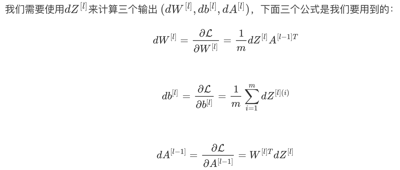
根据这三个公式来构建后向传播函数

def linear_backward(dZ,cache):
    """
    为单层实现反向传播的线性部分（第L层）

    参数：
         dZ - 相对于（当前第l层的）线性输出的成本梯度
         cache - 来自当前层前向传播的值的元组（A_prev，W，b）

    返回：
         dA_prev - 相对于激活（前一层l-）的成本梯度，与A_prev维度相同
         dW - 相对于W（当前层l）的成本梯度，与W的维度相同
         db - 相对于b（当前层l）的成本梯度，与b维度相同
    """
    A_prev, W, b = cache
    m = A_prev.shape[]
    dW = np.dot(dZ, A_prev.T) / m
    db = np.sum(dZ, axis=, keepdims=True) / m
    dA_prev = np.dot(W.T, dZ)

    assert (dA_prev.shape == A_prev.shape)
    assert (dW.shape == W.shape)
    assert (db.shape == b.shape)

    return dA_prev, dW, db

测试函数：

def linear_backward_test_case(): #随机生成前向传播结果用于测试后向
    """
    z, linear_cache = (np.array([[-0.8019545 ,  3.85763489]]), (np.array([[-1.02387576,  1.12397796],
       [-1.62328545,  0.64667545],
       [-1.74314104, -0.59664964]]), np.array([[ 0.74505627,  1.97611078, -1.24412333]]), np.array([[]]))
    """
    np.random.seed()
    dZ = np.random.randn(,)
    A = np.random.randn(,)
    W = np.random.randn(,)
    b = np.random.randn(,)
    linear_cache = (A, W, b)
    return dZ, linear_cache

测试：

#测试linear_backward
print("==============测试linear_backward==============")
dZ, linear_cache = testCases.linear_backward_test_case()

dA_prev, dW, db = linear_backward(dZ, linear_cache)
print ("dA_prev = "+ str(dA_prev))
print ("dW = " + str(dW))
print ("db = " + str(db))

返回：

==============测试linear_backward==============
dA_prev = [[ 0.51822968 -0.19517421]
 [-0.40506361  0.15255393]
 [ 2.37496825 -0.89445391]]
dW = [[-0.10076895  1.40685096  1.64992505]]
db = [[0.50629448]]

2）线性激活部分

将线性部分也使用了进来

在dnn_utils.py中定义了两个现成可用的后向函数，用来帮助计算dz：

如果 g(.)是激活函数, 那么sigmoid_backward 和 relu_backward 这样计算：

• sigmoid_backward:实现了sigmoid（）函数的反向传播，用来计算dz为：

dZ = sigmoid_backward(dA, activation_cache)

• relu_backward: 实现了relu（）函数的反向传播，用来计算dz为：

dZ = relu_backward(dA, activation_cache)

后向函数为：

def sigmoid_backward(dA, cache):
    """
    Implement the backward propagation for a single SIGMOID unit.

    Arguments:
    dA -- post-activation gradient, of any shape
    cache -- 'Z' where we store for computing backward propagation efficiently

    Returns:
    dZ -- Gradient of the cost with respect to Z
    """

    Z = cache

    s = /(+np.exp(-Z))
    dZ = dA * s * (-s)

    assert (dZ.shape == Z.shape)

    return dZ

def relu_backward(dA, cache):
    """
    Implement the backward propagation for a single RELU unit.

    Arguments:
    dA -- post-activation gradient, of any shape
    cache -- 'Z' where we store for computing backward propagation efficiently

    Returns:
    dZ -- Gradient of the cost with respect to Z
    """

    Z = cache
    dZ = np.array(dA, copy=True) # just converting dz to a correct object.

    # When z <= , you should set dz to  as well.
    dZ[Z <= ] = 

    assert (dZ.shape == Z.shape)

    return dZ

代码为：

def linear_activation_backward(dA,cache,activation="relu"):
    """
    实现LINEAR-> ACTIVATION层的后向传播。

    参数：
         dA - 当前层l的激活后的梯度值
         cache - 我们存储的用于有效计算反向传播的值的元组（值为linear_cache，activation_cache）
         activation - 要在此层中使用的激活函数名，字符串类型，【"sigmoid" | "relu"】
    返回：
         dA_prev - 相对于激活（前一层l-）的成本梯度值，与A_prev维度相同
         dW - 相对于W（当前层l）的成本梯度值，与W的维度相同
         db - 相对于b（当前层l）的成本梯度值，与b的维度相同
    """
    linear_cache, activation_cache = cache
    #其实是先通过线性激活部分后向传播得到dz，然后再将dz带入线性部分的后向传播得到dw,db,dA_prev
    if activation == "relu":
        dZ = relu_backward(dA, activation_cache)
        dA_prev, dW, db = linear_backward(dZ, linear_cache)
    elif activation == "sigmoid":
        dZ = sigmoid_backward(dA, activation_cache)
        dA_prev, dW, db = linear_backward(dZ, linear_cache)

    return dA_prev,dW,db

测试函数为：

def linear_activation_backward_test_case():
    """
    aL, linear_activation_cache = (np.array([[ 3.1980455 ,  7.85763489]]), ((np.array([[-1.02387576,  1.12397796], [-1.62328545,  0.64667545], [-1.74314104, -0.59664964]]), np.array([[ 0.74505627,  1.97611078, -1.24412333]]), ), np.array([[ 3.1980455 ,  7.85763489]])))
    """
    np.random.seed()
    dA = np.random.randn(,) #后向传播的输入
    A = np.random.randn(,) #存于cache中用于后向传播计算的值
    W = np.random.randn(,)
    b = np.random.randn(,)
    Z = np.random.randn(,)
    linear_cache = (A, W, b)
    activation_cache = Z
    linear_activation_cache = (linear_cache, activation_cache)

    return dA, linear_activation_cache

测试：

#测试linear_activation_backward
print("==============测试linear_activation_backward==============")
AL, linear_activation_cache = testCases.linear_activation_backward_test_case()

dA_prev, dW, db = linear_activation_backward(AL, linear_activation_cache, activation = "sigmoid")
print ("sigmoid:")
print ("dA_prev = "+ str(dA_prev))
print ("dW = " + str(dW))
print ("db = " + str(db) + "\n")

dA_prev, dW, db = linear_activation_backward(AL, linear_activation_cache, activation = "relu")
print ("relu:")
print ("dA_prev = "+ str(dA_prev))
print ("dW = " + str(dW))
print ("db = " + str(db))

返回：

==============测试linear_activation_backward==============
sigmoid:
dA_prev = [[ 0.11017994  0.01105339]
 [ 0.09466817  0.00949723]
 [-0.05743092 -0.00576154]]
dW = [[ 0.10266786  0.09778551 -0.01968084]]
db = [[-0.05729622]]

relu:
dA_prev = [[ 0.44090989 -.        ]
 [ 0.37883606 -.        ]
 [-0.2298228   .        ]]
dW = [[ 0.44513824  0.37371418 -0.10478989]]
db = [[-0.20837892]]

6.更新参数

根据上面后向传播得到的dw,db,dA_prev来更新参数，其中 α 是学习率

函数：

def update_parameters(parameters, grads, learning_rate):
    """
    使用梯度下降更新参数

    参数：
     parameters - 包含你的参数的字典，即w和b
     grads - 包含梯度值的字典，是L_model_backward的输出

    返回：
     parameters - 包含更新参数的字典
                   参数[“W”+ str（l）] = ...
                   参数[“b”+ str（l）] = ...
    """
    L = len(parameters) // 2 #整除2，得到层数
    for l in range(L):
        parameters["W" + str(l + )] = parameters["W" + str(l + )] - learning_rate * grads["dW" + str(l + )]
        parameters["b" + str(l + )] = parameters["b" + str(l + )] - learning_rate * grads["db" + str(l + )]

    return parameters

测试函数：

def update_parameters_test_case():
    """
    parameters = {'W1': np.array([[ 1.78862847,  0.43650985,  0.09649747],
        [-1.8634927 , -0.2773882 , -0.35475898],
        [-0.08274148, -0.62700068, -0.04381817],
        [-0.47721803, -1.31386475,  0.88462238]]),
 'W2': np.array([[ 0.88131804,  1.70957306,  0.05003364, -0.40467741],
        [-0.54535995, -1.54647732,  0.98236743, -1.10106763],
        [-1.18504653, -0.2056499 ,  1.48614836,  0.23671627]]),
 'W3': np.array([[-1.02378514, -0.7129932 ,  0.62524497],
        [-0.16051336, -0.76883635, -0.23003072]]),
 'b1': np.array([[ .],
        [ .],
        [ .],
        [ .]]),
 'b2': np.array([[ .],
        [ .],
        [ .]]),
 'b3': np.array([[ .],
        [ .]])}
    grads = {'dW1': np.array([[ 0.63070583,  0.66482653,  0.18308507],
        [ .        ,  .        ,  .        ],
        [ .        ,  .        ,  .        ],
        [ .        ,  .        ,  .        ]]),
 'dW2': np.array([[ 1.62934255,  .        ,  .        ,  .        ],
        [ .        ,  .        ,  .        ,  .        ],
        [ .        ,  .        ,  .        ,  .        ]]),
 'dW3': np.array([[-1.40260776,  .        ,  .        ]]),
 'da1': np.array([[ 0.70760786,  0.65063504],
        [ 0.17268975,  0.15878569],
        [ 0.03817582,  0.03510211]]),
 'da2': np.array([[ 0.39561478,  0.36376198],
        [ 0.7674101 ,  0.70562233],
        [ 0.0224596 ,  0.02065127],
        [-0.18165561, -0.16702967]]),
 'da3': np.array([[ 0.44888991,  0.41274769],
        [ 0.31261975,  0.28744927],
        [-0.27414557, -0.25207283]]),
 'db1': 0.75937676204411464,
 'db2': 0.86163759922811056,
 'db3': -0.84161956022334572}
    """
    np.random.seed()
    W1 = np.random.randn(,)
    b1 = np.random.randn(,)
    W2 = np.random.randn(,)
    b2 = np.random.randn(,)
    parameters = {"W1": W1,
                  "b1": b1,
                  "W2": W2,
                  "b2": b2}
    np.random.seed()
    dW1 = np.random.randn(,)
    db1 = np.random.randn(,)
    dW2 = np.random.randn(,)
    db2 = np.random.randn(,)
    grads = {"dW1": dW1,
             "db1": db1,
             "dW2": dW2,
             "db2": db2}

    return parameters, grads

测试：

#测试update_parameters
print("==============测试update_parameters==============")
parameters, grads = testCases.update_parameters_test_case()
parameters = update_parameters(parameters, grads, 0.1)

print ("W1 = "+ str(parameters["W1"]))
print ("b1 = "+ str(parameters["b1"]))
print ("W2 = "+ str(parameters["W2"]))
print ("b2 = "+ str(parameters["b2"]))

返回：

==============测试update_parameters==============
W1 = [[-0.59562069 -0.09991781 -2.14584584  1.82662008]
 [-1.76569676 -0.80627147  0.51115557 -1.18258802]
 [-1.0535704  -0.86128581  0.68284052  2.20374577]]
b1 = [[-0.04659241]
 [-1.28888275]
 [ 0.53405496]]
W2 = [[-0.55569196  0.0354055   1.32964895]]
b2 = [[-0.84610769]]

7.整合函数——训练

开始训练数据并得到最优参数

def two_layer_model(X,Y,layers_dims,learning_rate=0.0075,num_iterations=,print_cost=False,isPlot=True):
    """
    实现一个两层的神经网络，【LINEAR->RELU】 -> 【LINEAR->SIGMOID】
    参数：
        X - 输入的数据，维度为(n_x，例子数)
        Y - 标签，向量，0为非猫，1为猫，维度为(,数量)
        layers_dims - 层数的向量，维度为(n_y,n_h,n_y)
        learning_rate - 学习率
        num_iterations - 迭代的次数
        print_cost - 是否打印成本值，每100次打印一次
        isPlot - 是否绘制出误差值的图谱
    返回:
        parameters - 一个包含W1，b1，W2，b2的字典变量
    """
    np.random.seed()
    grads = {}
    costs = []
    (n_x,n_h,n_y) = layers_dims

    """
    初始化参数
    """
    parameters = initialize_parameters(n_x, n_h, n_y)

    W1 = parameters["W1"]
    b1 = parameters["b1"]
    W2 = parameters["W2"]
    b2 = parameters["b2"]

    """
    开始进行迭代
    """
    for i in range(,num_iterations):
        #前向传播
        A1, cache1 = linear_activation_forward(X, W1, b1, "relu")
        A2, cache2 = linear_activation_forward(A1, W2, b2, "sigmoid")

        #计算成本
        cost = compute_cost(A2,Y)

        #后向传播
        ##初始化后向传播
        dA2 = - (np.divide(Y, A2) - np.divide( - Y,  - A2))

        ##向后传播，输入：“dA2，cache2，cache1”。 输出：“dA1，dW2，db2;还有dA0（未使用），dW1，db1”。
        dA1, dW2, db2 = linear_activation_backward(dA2, cache2, "sigmoid")
        dA0, dW1, db1 = linear_activation_backward(dA1, cache1, "relu")

        ##向后传播完成后的数据保存到grads
        grads["dW1"] = dW1
        grads["db1"] = db1
        grads["dW2"] = dW2
        grads["db2"] = db2

        #更新参数
        parameters = update_parameters(parameters,grads,learning_rate)
        W1 = parameters["W1"]
        b1 = parameters["b1"]
        W2 = parameters["W2"]
        b2 = parameters["b2"]

        #打印成本值，如果print_cost=False则忽略
        if i %  == :
            #记录成本
            costs.append(cost)
            #是否打印成本值
            if print_cost:
                print("第", i ,"次迭代，成本值为：" ,np.squeeze(cost))
    #迭代完成，根据条件绘制图
    if isPlot:
        plt.plot(np.squeeze(costs))
        plt.ylabel('cost')
        plt.xlabel('iterations (per tens)')
        plt.title("Learning rate =" + str(learning_rate))
        plt.show()

    #返回parameters
    return parameters

我们现在开始加载数据集,图像数据集的处理可以参照吴恩达课后作业学习1-week2-homework-logistic

train_set_x_orig , train_set_y , test_set_x_orig , test_set_y , classes = lr_utils.load_dataset()

train_x_flatten = train_set_x_orig.reshape(train_set_x_orig.shape[], -).T
test_x_flatten = test_set_x_orig.reshape(test_set_x_orig.shape[], -).T

train_x = train_x_flatten /
train_y = train_set_y
test_x = test_x_flatten /
test_y = test_set_y

数据集加载完成，开始正式训练：

n_x =
n_h =
n_y =
layers_dims = (n_x,n_h,n_y)

parameters = two_layer_model(train_x, train_set_y, layers_dims = (n_x, n_h, n_y), num_iterations = , print_cost=True,isPlot=True)

返回：

第  次迭代，成本值为： 0.6930497356599891
第  次迭代，成本值为： 0.6464320953428849
第  次迭代，成本值为： 0.6325140647912678
第  次迭代，成本值为： 0.6015024920354665
第  次迭代，成本值为： 0.5601966311605748
第  次迭代，成本值为： 0.515830477276473
第  次迭代，成本值为： 0.47549013139433266
第  次迭代，成本值为： 0.4339163151225749
第  次迭代，成本值为： 0.40079775362038866
第  次迭代，成本值为： 0.3580705011323798
第  次迭代，成本值为： 0.33942815383664127
第  次迭代，成本值为： 0.30527536361962654
第  次迭代，成本值为： 0.2749137728213016
第  次迭代，成本值为： 0.2468176821061485
第  次迭代，成本值为： 0.19850735037466094
第  次迭代，成本值为： 0.17448318112556652
第  次迭代，成本值为： 0.17080762978096245
第  次迭代，成本值为： 0.11306524562164728
第  次迭代，成本值为： 0.09629426845937152
第  次迭代，成本值为： 0.08342617959726863
第  次迭代，成本值为： 0.07439078704319081
第  次迭代，成本值为： 0.06630748132267934
第  次迭代，成本值为： 0.05919329501038173
第  次迭代，成本值为： 0.05336140348560557
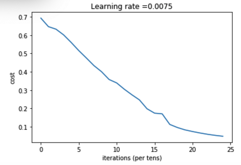
第  次迭代，成本值为： 0.048554785628770185

图示：

8.预测

def predict(X, y, parameters):
    """
    该函数用于预测L层神经网络的结果，当然也包含两层

    参数：
     X - 测试集
     y - 标签
     parameters - 训练模型得到的最优参数

    返回：
     p - 给定数据集X的预测
    """

    m = X.shape[]
    n = len(parameters) // 2 # 神经网络的层数
    p = np.zeros((,m))

    #根据参数前向传播
    probas, caches = L_model_forward(X, parameters)

    for i in range(, probas.shape[]):
        if probas[,i] > 0.5:
            p[,i] =
        else:
            p[,i] = 

    print("准确度为: "  + str(float(np.sum((p == y))/m)))

    return p

预测函数构建好了我们就开始预测，查看训练集和测试集的准确性：

predictions_train = predict(train_x, train_y, parameters) #训练集
predictions_test = predict(test_x, test_y, parameters) #测试集

返回：

准确度为: 1.0
准确度为: 0.72

可见两层的训练效果比单层的logistic回归的效果要好一些