GBDT,随机森林

author:yangjing

time:2018-10-22

---

Gradient boosting decision tree

1.main diea

The main idea behind GBDT is to combine many simple models(also known as week kernels),like shallow trees.Each tree can only provide good predictions on part of the data,and so more and more trees are added to iteratively improve performance.

2.parameters setting

the algorithm is a bit more sensitive to parameter settings than random forests,but can provide better accuracy if the parameters are set correctly.

• number of trees
  
  By increasing n_estimators ,also increasing the model complexity,as the model has more chances to correct misticks on the training set.
• learning rate
  
  controns how strongly each tree tries to correct the misticks of the previous trees.A higher learning rate means each tree can make stronger correctinos,allowing for more complex models.
• max_depth
  
  or alternatively max_leaf_nodes.Usyally max_depth is set very low for gradient-boosted models,often not deeper than five splits.

---

3.code

from sklearn.ensemble import GradientBoostingClassifier
from sklearn.model_selection import train_test_split
from sklearn.datasets import load_breast_cancer
cancer=load_breast_cancer()
X_train,X_test,y_train,y_test=train_test_split(cancer.data,cancer.target,random_state=0)
gbrt=GradientBoostingClassifier(random_state=0)
gbrt.fit(X_train,y_train)
gbrt.score(X_test,y_test)

In [261]: X_train,X_test,y_train,y_test=train_test_split(cancer.data,cancer.target,random_state=0)
     ...: gbrt=GradientBoostingClassifier(random_state=0)
     ...: gbrt.fit(X_train,y_train)
     ...: gbrt.score(X_test,y_test)
     ...:
Out[261]: 0.958041958041958

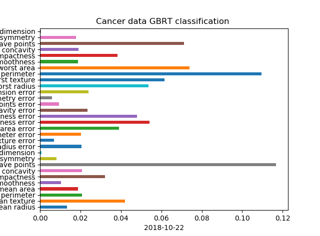
In [262]: gbrt.feature_importances_
Out[262]:
array([0.01337291, 0.04201687, 0.0208666 , 0.01889077, 0.01028091,
       0.03215986, 0.02074619, 0.11678956, 0.00820024, 0.00074312,
       0.02042134, 0.00680047, 0.02023052, 0.03907398, 0.05406751,
       0.04795741, 0.02358101, 0.00934718, 0.00593481, 0.0239241 ,
       0.05354265, 0.06160083, 0.10961728, 0.07395201, 0.01867851,
       0.03842953, 0.01915824, 0.07128703, 0.01773659, 0.00059199])

In [263]: gbrt.learning_rate
Out[263]: 0.1

In [264]: gbrt.max_depth
Out[264]: 3

In [265]: len(gbrt.estimators_)
Out[266]: 100

In [272]: gbrt.get_params()
Out[272]:
{'criterion': 'friedman_mse',
 'init': None,
 'learning_rate': 0.1,
 'loss': 'deviance',
 'max_depth': 3,
 'max_features': None,
 'max_leaf_nodes': None,
 'min_impurity_decrease': 0.0,
 'min_impurity_split': None,
 'min_samples_leaf': 1,
 'min_samples_split': 2,
 'min_weight_fraction_leaf': 0.0,
 'n_estimators': 100,
 'presort': 'auto',
 'random_state': 0,
 'subsample': 1.0,
 'verbose': 0,
 'warm_start': False}

---

Random forest

In [230]: y
Out[230]:
array([1, 1, 0, 1, 1, 1, 1, 0, 0, 0, 1, 0, 1, 1, 0, 1, 1, 0, 1, 0, 1, 0,
       0, 0, 1, 1, 0, 1, 0, 1, 0, 0, 0, 0, 1, 0, 1, 1, 0, 0, 0, 0, 0, 0,
       1, 1, 1, 1, 1, 0, 1, 1, 1, 1, 0, 1, 1, 1, 1, 1, 0, 1, 1, 1, 0, 1,
       0, 0, 0, 0, 0, 1, 1, 0, 1, 1, 0, 1, 1, 0, 1, 0, 1, 0, 0, 0, 0, 0,
       0, 1, 0, 0, 1, 0, 0, 0, 1, 1, 0, 0], dtype=int64)

In [231]: axes.ravel()
Out[231]:
array([<matplotlib.axes._subplots.AxesSubplot object at 0x000001F46F3694A8>,
       <matplotlib.axes._subplots.AxesSubplot object at 0x000001F46C099F28>,
       <matplotlib.axes._subplots.AxesSubplot object at 0x000001F46E6E3BE0>,
       <matplotlib.axes._subplots.AxesSubplot object at 0x000001F46BEB72E8>,
       <matplotlib.axes._subplots.AxesSubplot object at 0x000001F46ED67198>,
       <matplotlib.axes._subplots.AxesSubplot object at 0x000001F46F292C88>],
      dtype=object)

In [232]: from sklearn.model_selection import train_test_split

In [233]: X_trai,X_test,y_train,y_test=train_test_split(X,y,stratify=y,random_state=42)

In [234]: len(X_trai)
Out[234]: 75

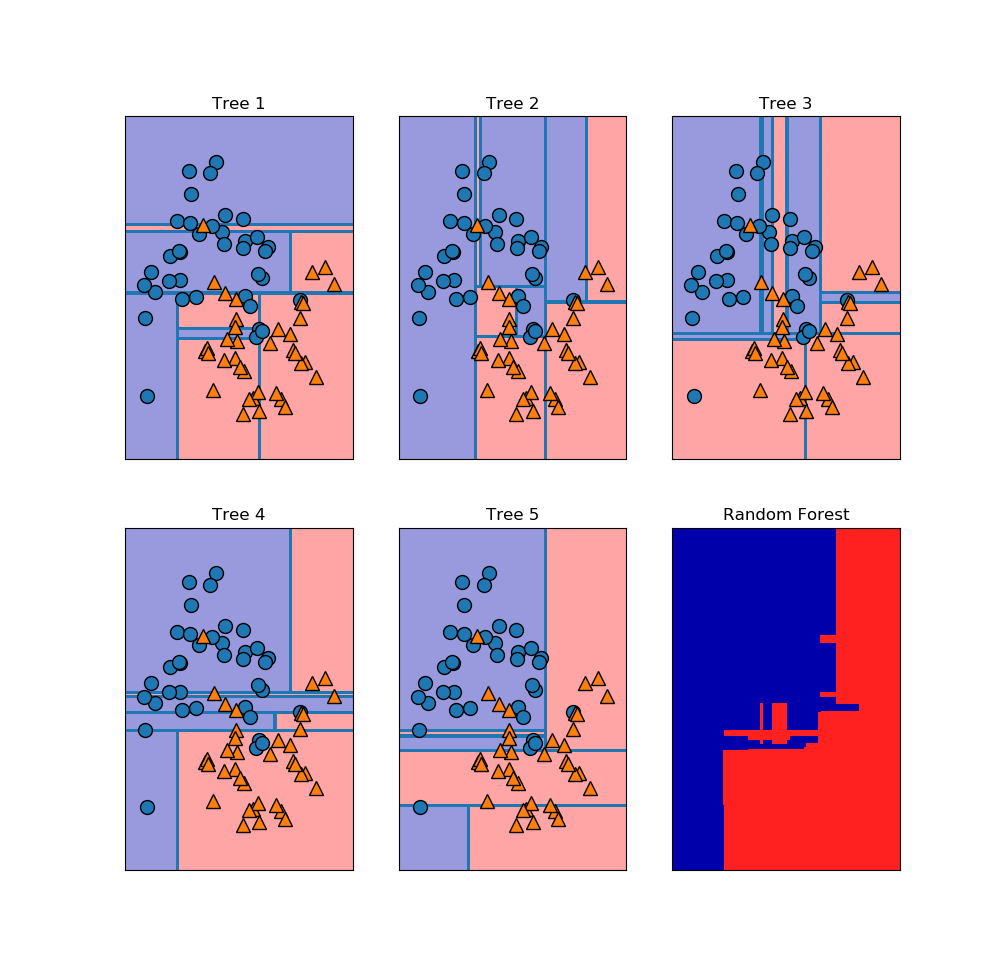
In [235]: fores=RandomForestClassifier(n_estimators=5,random_state=2)

In [236]: fores.fit(X_trai,y_train)
Out[236]:
RandomForestClassifier(bootstrap=True, class_weight=None, criterion='gini',
            max_depth=None, max_features='auto', max_leaf_nodes=None,
            min_impurity_decrease=0.0, min_impurity_split=None,
            min_samples_leaf=1, min_samples_split=2,
            min_weight_fraction_leaf=0.0, n_estimators=5, n_jobs=1,
            oob_score=False, random_state=2, verbose=0, warm_start=False)

In [237]: fores.score(X_test,y_test)
Out[237]: 0.92

In [238]: fores.estimators_
Out[238]:
[DecisionTreeClassifier(class_weight=None, criterion='gini', max_depth=None,
             max_features='auto', max_leaf_nodes=None,
             min_impurity_decrease=0.0, min_impurity_split=None,
             min_samples_leaf=1, min_samples_split=2,
             min_weight_fraction_leaf=0.0, presort=False,
             random_state=1872583848, splitter='best'),
 DecisionTreeClassifier(class_weight=None, criterion='gini', max_depth=None,
             max_features='auto', max_leaf_nodes=None,
             min_impurity_decrease=0.0, min_impurity_split=None,
             min_samples_leaf=1, min_samples_split=2,
             min_weight_fraction_leaf=0.0, presort=False,
             random_state=794921487, splitter='best'),
 DecisionTreeClassifier(class_weight=None, criterion='gini', max_depth=None,
             max_features='auto', max_leaf_nodes=None,
             min_impurity_decrease=0.0, min_impurity_split=None,
             min_samples_leaf=1, min_samples_split=2,
             min_weight_fraction_leaf=0.0, presort=False,
             random_state=111352301, splitter='best'),
 DecisionTreeClassifier(class_weight=None, criterion='gini', max_depth=None,
             max_features='auto', max_leaf_nodes=None,
             min_impurity_decrease=0.0, min_impurity_split=None,
             min_samples_leaf=1, min_samples_split=2,
             min_weight_fraction_leaf=0.0, presort=False,
             random_state=1853453896, splitter='best'),
 DecisionTreeClassifier(class_weight=None, criterion='gini', max_depth=None,
             max_features='auto', max_leaf_nodes=None,
             min_impurity_decrease=0.0, min_impurity_split=None,
             min_samples_leaf=1, min_samples_split=2,
             min_weight_fraction_leaf=0.0, presort=False,
             random_state=213298710, splitter='best')]