Candidate Generation and LUNA16 preprocessing

在这个kernel中，我们将讨论有助于更好地理解问题陈述和数据可视化的方法。 我还将提供有用的资源和信息的链接。

此脚本是用Python编写的。 我建议人们在桌面上安装anaconda，因为here提到了它的优点。 本教程中用于读取，处理和可视化数据的库是matplotlib，numpy，skimage和pydicom.。

图像大小（z，512,512），其中z是CT扫描中的切片数量，取决于扫描仪的分辨率。 由于计算能力的限制，这样的大图像不能直接送到卷积网络中。 因此，我们将不得不找到更可能患有癌症的地区。 我们将通过首先分割肺部，然后去除低强度区域来缩小我们的搜索空间。

在本教程中，我们将首先读入数据集并对其进行可视化。 之后，我们将分割肺部结构，然后使用图像处理方法在CT扫描中找到感兴趣的区域（可能的癌症区域）。 接下来我将介绍如何预处理LUNA16数据集，用于UNet等训练架构的分割和候选分类。

肺结构的分割是非常具有挑战性的问题，因为在肺部区域不存在同质性，在肺部结构，不同扫描仪和扫描协议中密度相似。 分割的肺可以进一步用于发现肺部结节候选者和感兴趣的区域，这可能有助于更好地分类CT扫描。 发现肺结节区域是一个非常困难的问题，因为附着在血管上的结节或者存在于肺区域的边界处。 肺结节候选者可以通过切割周围的三维体素并通过可以在LUNA16数据集上训练的3D CNNs进一步用于分类。 LUNA 16数据集具有每个CT扫描中的结节的位置，因此对于训练分类器将是有用的。

Reading a CT Scan

输入文件夹有三件事，一个是sample_images文件夹，它具有CT扫描样本。 stage1_labels.csv包含阶段1训练集图像的癌症基础事实，stage1_sample_submission.csv显示阶段1的提交格式。

In [1]:

# This Python 3 environment comes with many helpful analytics libraries installed
# It is defined by the kaggle/python docker image: https://github.com/kaggle/docker-python
# For example, here's several helpful packages to load in 

import numpy as np # linear algebra
import pandas as pd # data processing, CSV file I/O (e.g. pd.read_csv)
import skimage, os
from skimage.morphology import ball, disk, dilation, binary_erosion, remove_small_objects, erosion, closing, reconstruction, binary_closing
from skimage.measure import label,regionprops, perimeter
from skimage.morphology import binary_dilation, binary_opening
from skimage.filters import roberts, sobel
from skimage import measure, feature
from skimage.segmentation import clear_border
from skimage import data
from scipy import ndimage as ndi
import matplotlib.pyplot as plt
from mpl_toolkits.mplot3d.art3d import Poly3DCollection
import dicom
import scipy.misc
import numpy as np

# Input data files are available in the "../input/" directory.
# For example, running this (by clicking run or pressing Shift+Enter) will list the files in the input directory

from subprocess import check_output
print(check_output(["ls", "../input"]).decode("utf8"))
#上面两句话是无法在windows下执行的（没有ls的binay文件）
import os

cwd = os.getcwd()
file_path=cwd+'/input'
print(os.listdir(file_path))

结果：

['sample_images', 'stage1_labels.csv', 'stage1_sample_submission.csv']

每个三维CT扫描由多个切片组成，其数目取决于扫描仪的分辨率，每个切片都有一个与之关联的实例号，它告诉从顶部切片的索引。 CT扫描的所有dicom文件都在CT扫描名称的一个文件夹内。 现在我们将读取扫描的所有dicom切片，然后根据它们的实例编号堆叠它们以获得3D肺部CT扫描图像。

sample_images文件夹大约有20个文件夹，每个文件夹对应一个CT扫描。 在文件夹里面有很多dicom文件。

In [2]:

image_path=file_path+'/sample_images'
print(os.listdir(image_path))

结果：

['00cba091fa4ad62cc3200a657aeb957e', '0a099f2549429d29b32f349e95fb2244', '0a0c32c9e08cc2ea76a71649de56be6d', '0a38e7597ca26f9374f8ea2770ba870d', '0acbebb8d463b4b9ca88cf38431aac69', '0b20184e0cd497028bdd155d9fb42dc9', '0bd0e3056cbf23a1cb7f0f0b18446068', '0c0de3749d4fe175b7a5098b060982a1', '0c37613214faddf8701ca41e6d43f56e', '0c59313f52304e25d5a7dcf9877633b1', '0c60f4b87afcb3e2dfa65abbbf3ef2f9', '0c98fcb55e3f36d0c2b6507f62f4c5f1', '0c9d8314f9c69840e25febabb1229fa4', '0ca943d821204ceb089510f836a367fd', '0d06d764d3c07572074d468b4cff954f', '0d19f1c627df49eb223771c28548350e', '0d2fcf787026fece4e57be167d079383', '0d941a3ad6c889ac451caf89c46cb92a', '0ddeb08e9c97227853422bd71a2a695e', '0de72529c30fe642bc60dcb75c87f6bd']

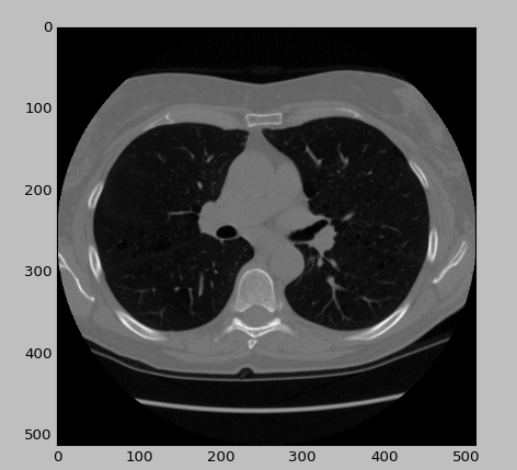
每个CT扫描由多个以DICOM格式提供的2D切片组成。 首先，我将读取CT扫描的随机dicom文件。 读取图像文件后，我们将用0更新-2000的亮度值，因为它们是落在扫描仪边界之外的像素。

# Any results you write to the current directory are saved as output.
def loadFileInformation(filename):
    information = {}
    ds = dicom.read_file(filename)
    information['PatientID'] = ds.PatientID
    information['PatientName'] = ds.PatientName
    information['PatientBirthDate'] = ds.PatientBirthDate
    return information

random_dcm_path=image_path+'/00cba091fa4ad62cc3200a657aeb957e/38c4ff5d36b5a6b6dc025435d62a143d.dcm'
# print(loadFileInformation(random_dcm_path))
lung = dicom.read_file(random_dcm_path)

slice = lung.pixel_array
slice[slice == -2000] = 0
plt.imshow(slice, cmap=plt.cm.gray)
plt.show()

结果：

def read_ct_scan(folder_name):
    # Read the slices from the dicom file
    slices = [dicom.read_file(folder_name + '/'+filename) for filename in os.listdir(folder_name)]

    # Sort the dicom slices in their respective order
    slices.sort(key=lambda x: int(x.InstanceNumber))

    # Get the pixel values for all the slices
    slices = np.stack([s.pixel_array for s in slices])
    slices[slices == -2000] = 0
    return slices
某个病人CT_path=image_path+'/00cba091fa4ad62cc3200a657aeb957e'
ct_scan = read_ct_scan(某个病人CT_path)

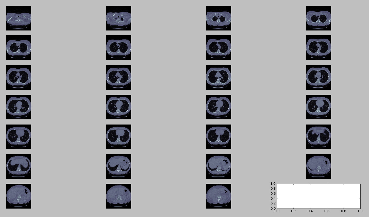
为了可视化切片，我们将必须绘制它们。 matplotlib用于绘制切片。 plot_ct_scan函数将三维CT扫描图像数组作为输入，并绘制等间距切片。 CT扫描是灰度图像，即每个像素的值是单个样本，这意味着它仅携带强度信息。

def plot_ct_scan(scan):
    f, plots = plt.subplots(int(scan.shape[0] / 20) + 1, 4, figsize=(25, 25))
    for i in range(0, scan.shape[0], 5):
        plots[int(i / 20), int((i % 20) / 5)].axis('off')
        plots[int(i / 20), int((i % 20) / 5)].imshow(scan[i], cmap=plt.cm.bone)
plot_ct_scan(ct_scan)
plt.show()

结果：

Segmentation of Lungs

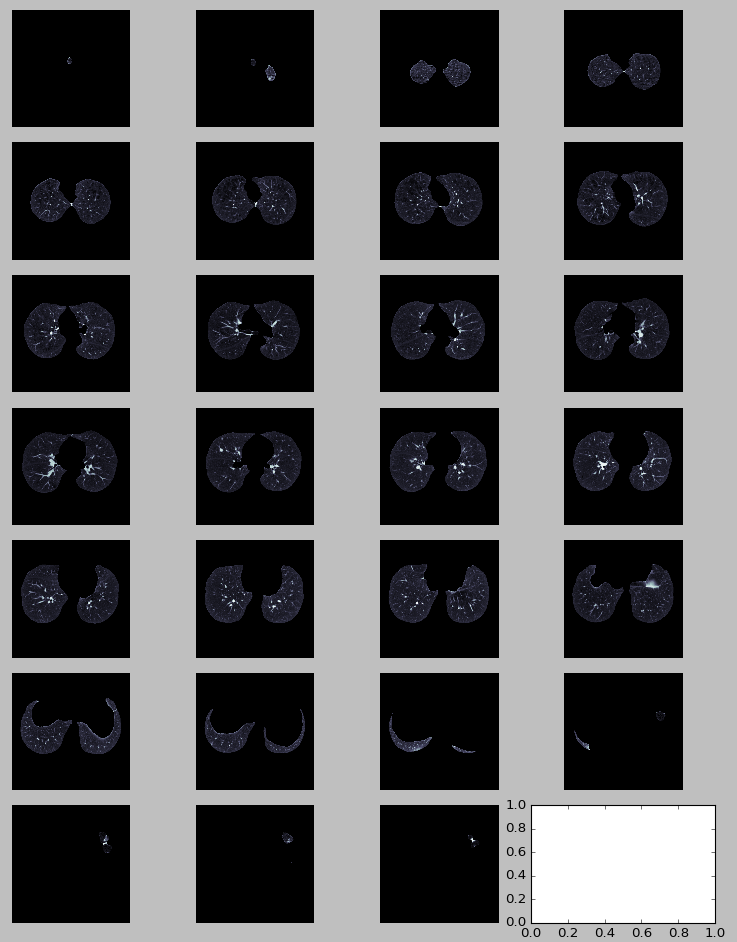
在阅读CT扫描之后，预处理的第一步就是肺结构的分割，因为显然感兴趣的区域位于肺内。 可以看出，肺部是CT扫描中较暗的区域。 肺内的明亮区域是血管或空气。 在所有地方使用604（-400HU）的阈值，因为在实验中发现它工作得很好。 我们从CT扫描图像的每个切片中分割出肺部结构，尽量不要放过附着在肺壁上的可能区域。 有一些可能附着在肺壁上的结节。

我将首先解释一个常见的方法，使用简单的图像处理和形态学操作来分割肺部，然后将给文献的良好链接提供参考和总结。

def get_segmented_lungs(im, plot=False):
    '''
    This funtion segments the lungs from the given 2D slice.
    '''
    if plot == True:
        f, plots = plt.subplots(8, 1, figsize=(5, 40))
    '''
    Step 1: Convert into a binary image.
    '''
    binary = im < 604
    if plot == True:
        plots[0].axis('off')
        plots[0].imshow(binary, cmap=plt.cm.bone)
    '''
    Step 2: Remove the blobs connected to the border of the image.
    '''
    cleared = clear_border(binary)
    if plot == True:
        plots[1].axis('off')
        plots[1].imshow(cleared, cmap=plt.cm.bone)
    '''
    Step 3: Label the image.
    '''
    label_image = label(cleared)
    if plot == True:
        plots[2].axis('off')
        plots[2].imshow(label_image, cmap=plt.cm.bone)
    '''
    Step 4: Keep the labels with 2 largest areas.
    '''
    areas = [r.area for r in regionprops(label_image)]
    areas.sort()
    if len(areas) > 2:
        for region in regionprops(label_image):
            if region.area < areas[-2]:
                for coordinates in region.coords:
                    label_image[coordinates[0], coordinates[1]] = 0
    binary = label_image > 0
    if plot == True:
        plots[3].axis('off')
        plots[3].imshow(binary, cmap=plt.cm.bone)
    '''
    Step 5: Erosion operation with a disk of radius 2. This operation is
    seperate the lung nodules attached to the blood vessels.
    '''
    selem = disk(2)
    binary = binary_erosion(binary, selem)
    if plot == True:
        plots[4].axis('off')
        plots[4].imshow(binary, cmap=plt.cm.bone)
    '''
    Step 6: Closure operation with a disk of radius 10. This operation is
    to keep nodules attached to the lung wall.
    '''
    selem = disk(10)
    binary = binary_closing(binary, selem)
    if plot == True:
        plots[5].axis('off')
        plots[5].imshow(binary, cmap=plt.cm.bone)
    '''
    Step 7: Fill in the small holes inside the binary mask of lungs.
    '''
    edges = roberts(binary)
    binary = ndi.binary_fill_holes(edges)
    if plot == True:
        plots[6].axis('off')
        plots[6].imshow(binary, cmap=plt.cm.bone)
    '''
    Step 8: Superimpose the binary mask on the input image.
    '''
    get_high_vals = binary == 0
    im[get_high_vals] = 0
    if plot == True:
        plots[7].axis('off')
        plots[7].imshow(im, cmap=plt.cm.bone)

    return im

get_segmented_lungs函数分割CT扫描的二维切片。 为了更好的可视化和理解代码和应用操作，我已经输出切片。

get_segmented_lungs(ct_scan[71], True)
plt.show()

结果：

现在，我将逐片分割整个CT扫描并显示CT扫描的一些切片。

def segment_lung_from_ct_scan(ct_scan):
    return np.asarray([get_segmented_lungs(slice) for slice in ct_scan])

segmented_ct_scan = segment_lung_from_ct_scan(ct_scan)
plot_ct_scan(segmented_ct_scan)
plt.show()

结果：

Nodule Candidate/Region of Interest Generation

在从CT扫描图像中分割出肺部结构之后，我们的任务是找到具有结节的候选区域，因为搜索空间非常大。 而且由于计算的局限性，整幅图像不能直接用3D CNNs进行分类，需要找到可能的癌症区域并对其进行分类。 在实验中发现，所有的兴趣区域的强度> 604（-400 HU）。 所以，我们使用这个阈值来过滤较暗的区域。 这大大减少了候选人数量，保留了召回率高的重要区域。 然后我们将所有候选点分类以减少误报。

segmented_ct_scan[segmented_ct_scan < 604] = 0
plot_ct_scan(segmented_ct_scan)
plt.show()

结果：

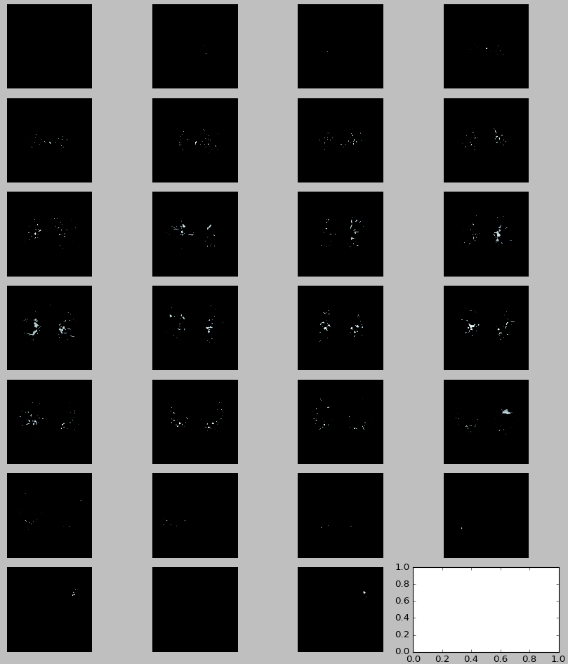
过滤后，由于血管仍然有很多噪音。 因此，我们进一步删除两个最大的连接组件（ remove the two largest connected component）。

selem = ball(2)
binary = binary_closing(segmented_ct_scan, selem)

label_scan = label(binary)

areas = [r.area for r in regionprops(label_scan)]
areas.sort()

for r in regionprops(label_scan):
    max_x, max_y, max_z = 0, 0, 0
    min_x, min_y, min_z = 1000, 1000, 1000

    for c in r.coords:
        max_z = max(c[0], max_z)
        max_y = max(c[1], max_y)
        max_x = max(c[2], max_x)

        min_z = min(c[0], min_z)
        min_y = min(c[1], min_y)
        min_x = min(c[2], min_x)
    if (min_z == max_z or min_y == max_y or min_x == max_x or r.area > areas[-3]):
        for c in r.coords:
            segmented_ct_scan[c[0], c[1], c[2]] = 0
    else:
        index = (max((max_x - min_x), (max_y - min_y), (max_z - min_z))) / (min((max_x - min_x), (max_y - min_y), (max_z - min_z)))

plot_3d函数绘制CT扫描的3D numpy数组。

In [14]:

def plot_3d(image, threshold=-300):
    # Position the scan upright,
    # so the head of the patient would be at the top facing the camera
    p = image.transpose(2, 1, 0)
    p = p[:, :, ::-1]

    verts, faces = measure.marching_cubes(p, threshold)

    fig = plt.figure(figsize=(10, 10))
    ax = fig.add_subplot(111, projection='3d')

    # Fancy indexing: `verts[faces]` to generate a collection of triangles
    mesh = Poly3DCollection(verts[faces], alpha=0.1)
    face_color = [0.5, 0.5, 1]
    mesh.set_facecolor(face_color)
    ax.add_collection3d(mesh)

    ax.set_xlim(0, p.shape[0])
    ax.set_ylim(0, p.shape[1])
    ax.set_zlim(0, p.shape[2])

In [15]:

plot_3d(segmented_ct_scan, 604)
plt.show()

结果：

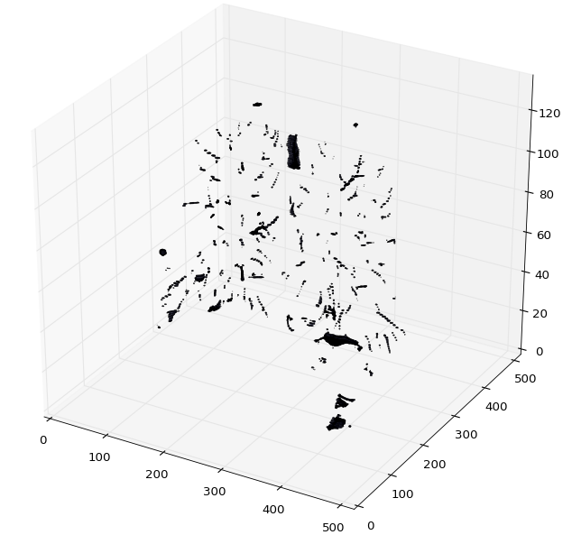
还有更多的方法可以去尝试获取感兴趣的区域。

　　1. 因为我们知道结节是球形的，所以左侧血管可以进一步使用形状特性进行过滤。

　　2. 可以进一步使用超像素（应该指的是加强分倍率）分割，并且可以在分割区域上应用形状属性。
　　3. 像UNet这样的CNN体系结构也可以用来生成候选感兴趣区域。

使用图像处理方法也有很多关于肺分割和结节候选生成的优秀论文。 我列出一些方法的小结：

1. Automatic segmentation of lung nodules with growing neural gas and support vector machine-所提出的方法包括采集肺的计算机断层扫描图像（CT），通过提取胸腔，提取肺和重建实质的原始形状的技术减少感兴趣的体积。 之后，使用生长的神经气体（GNG）来限制比肺实质更密集的结构（结节，血管，支气管等）。 下一个阶段是类似肺结节的结构与其他结构如血管和支气管的分离。 最后，通过形状和纹理测量以及支持向量机将结构分类为结核或非结核。
2. Automated Segmentation of Lung Regions using Morphological Operators in CT scan-get_segmented_lungs方法是这篇文章的一个小修改。 本文采用了604的门槛值。
3. Pre-processing methods for nodule detection in lung CT- 本文采用点增强滤波器应用于体素数据的三维矩阵。 该3D滤波器试图确定每个体素的局部几何特性，计算Hessian矩阵的特征值并评估特意构建的“似然”函数，以区分线性，平面和球形物体的局部形态，将其建模为具有3D高斯部分 （Q. Li，S. Sone和K. Doi [6]）。 通过将这种3D滤波器应用于人造图像，即使在将其叠加到非高斯区域的情况下，我们也验证了高斯样区域检测的效率。
4. Lung Nodule Detection using a Neural Classifier:本文讨论了用于结节候选选择的点增强滤波器和用于假阳性发现减少的神经分类器。 该性能被评估为全自动计算机化的方法，用于在筛查CT中识别可能在视觉解释期间遗漏的肺癌的肺结节的检测。

接下来我将讨论关于LUNA16数据集的预处理，并用它来训练UNet模型。

UNET for Candidate Point Generation

目前深度学习方法在医学影像分割问题上取得了较好的效果。 一个非常有名的建筑是UNET，在我们的例子中可以用于结节候选点生成。 这些网络的培训使用注释数据集完成。 上述用于候选点生成的图像处理方法不需要任何训练数据。 我们使用LUNA16数据集来训练我们的UNET模型。

在LUNA16数据集中，每个CT扫描用结节点和用于生成二进制掩模的结节的半径来标注。 我将首先讨论LUNA16数据集的预处理。 在数据集中，CT扫描保存在“.mhd”文件中，SimpleITK用于读取图像。 我已经定义了三个功能：