[ML] Load and preview large scale data

Ref: [Feature] Preprocessing tutorial

主要是 “无量纲化” 之前的部分。

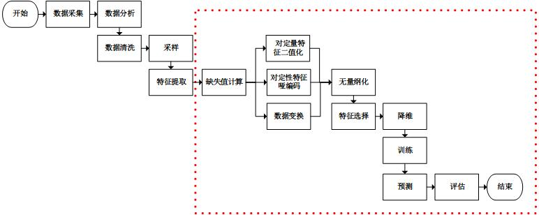
加载数据

一、大数据源

http://archive.ics.uci.edu/ml/
http://aws.amazon.com/publicdatasets/
http://www.kaggle.com/
http://www.kdnuggets.com/datasets/index.html

二、初步查看

了解需求

Swipejobs is all about matching Jobs to Workers. Your challenge is to analyse the data provided and answer the questions below.

You can access the data by opening the following S3 bucket:

/* somewhere */

Please note that Worker (worker parquet files) has one or more job tickets (jobticket parquet files) associated with it.

Using these parquet files:

求相关性
1. Is there a co-relation between jobticket.jobTicketState, jobticket.clickedCalloff and jobticket.assignedBySwipeJobs values across workers.

预测
2. Looking at Worker.profileLastUpdatedDate values, calculate an estimation for workers who will update their profile in the next two weeks.

requirement

Requirement

粗看数据

head -5 <file>
less <file>

三、数据读取

python读取txt文件

没有格式，就要split出格式，还是建议之后转到df格式，操作方便些。

PATH = "/home/ubuntu/work/rajdeepd-spark-ml/spark-ml/data"
user_data = sc.textFile("%s/ml-100k/u.user" % PATH)

user_fields = user_data.map(lambda line: line.split("|"))
print(user_fields)
user_fields.take(5)

PythonRDD[29] at RDD at PythonRDD.scala:53
  Out[19]:
[['', '', 'M', 'technician', ''],
 ['', '', 'F', 'other', ''],
 ['', '', 'M', 'writer', ''],
 ['', '', 'M', 'technician', ''],
 ['', '', 'F', 'other', '']]

python读取parquet文件

Spark SQL还是作为首选工具，参见：[Spark] 03 - Spark SQL

Ref: 读写parquet格式文件的几种方式

本文将介绍常用parquet文件读写的几种方式

1. 用spark的hadoopFile api 读取hive中的 parquet格式。
2. 用 sparkSql 读写hive中的parquet。
3. 用新旧MapReduce读写parquet格式文件。

4. 用 SparkSql 读写s3中的parquet。

Ref: How to read parquet data from S3 to spark dataframe Python?

spark = SparkSession.builder
                        .master("local")
                        .appName("app name")
                        .config("spark.some.config.option", true).getOrCreate()

df = spark.read.parquet("s3://path/to/parquet/file.parquet")

python读取csv文件

# define the schema, corresponding to a line in the csv data file.
schema = StructType([
    StructField("long", FloatType(), nullable=True),
    StructField("lat", FloatType(), nullable=True),
    StructField("medage", FloatType(), nullable=True),
    StructField("totrooms", FloatType(), nullable=True),
    StructField("totbdrms", FloatType(), nullable=True),
    StructField("pop", FloatType(), nullable=True),
    StructField("houshlds", FloatType(), nullable=True),
    StructField("medinc", FloatType(), nullable=True),
    StructField("medhv", FloatType(), nullable=True)]
)

schema

# 参数中包含了column的定义
housing_df = spark.read.csv(path=HOUSING_DATA, schema=schema).cache()

# User-friendly的表格显示
housing_df.show(5)

# 包括了列的性质
housing_df.printSchema()

四、数据库到HBase

MySQL (binlog) --> Maxwell --> Kafka --> HBase --> Parquet.

Ref: maxwell将mysql数据实时同步到kafka

Ref: MySQL Binlog 解析工具 Maxwell 详解

抛出问题

我们的业务数据存放在mysql中，但是在大数据系统中我们需要拿hbase的数据进行业务处理，比如推荐系统。

那么怎么可以将mysql中的业务数据实时同步到hbase中，从而可以在大数据系统中进行实时流式计算。

 

对应方案

(1) MySQL到HBase

本次推荐工具maxwell，方式是：我们打开mysql的binlog模式，数据以row为单位输出，然后通过maxwell发送给kafka，再由另一个程序将kafka数据录入到hbase中。

 

(2) HBase到Parquet

Ref: How to move HBase tables to HDFS in Parquet format?

Ref: spark 读 hbase parquet 哪个快

Spark读hbase，生成task受所查询table的region个数限制，任务数有限，例如查询的40G数据，10G一个region，很可能就4~6个region，初始的task数就只有4~6个左右，RDD后续可以partition设置task数；spark读parquet按默认的bolck个数生成task个数，例如128M一个bolck，差不多就是300多个task，初始载入情况就比hbase快，而且直接载入parquet文件到spark的内存，而hbase还需要同regionserver交互把数据传到spark的内存也是需要消耗时间的。

总体来说，读parquet更快。

了解数据

—— RDD方式，以及正统的高阶方法：[Spark] 03 - Spark SQL

一、初步清理数据

前期发现缺失数据、不合格的数据。

# 可用于检查“空数据”、“不合格的数据”
def convert_year(x):
    try:
        return int(x[-4:])
    except:
        return 1900 # there is a 'bad' data point with a blank year, which we set to 1900 and will filter out later

movie_fields = movie_data.map(lambda lines: lines.split("|"))
years = movie_fields.map(lambda fields: fields[2]).map(lambda x: convert_year(x)) 

二、特征内部类别数

num_genders     = user_fields.map(lambda fields: fields[2]).distinct().count()
num_occupations = user_fields.map(lambda fields: fields[3]).distinct().count()
num_zipcodes    = user_fields.map(lambda fields: fields[4]).distinct().count()

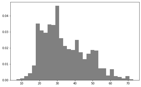
也就是下图中惨素hist中的bins的原始值。

三、某个特征可视化

是否符合正态分布，可视化后甄别“异常值”。

数据如果有偏，可以通过log转换。

plt.hist 方法

简单地，使用hist直接得到柱状图；如果数据量太大，可以先抽样，再显示。

import matplotlib.pyplot as plt

ages = user_fields.map(lambda x: int(x[1])).collect()
plt.hist(ages, bins=30, color='gray', normed=True)
fig = matplotlib.pyplot.gcf()
fig.set_size_inches(8, 5)

* Pandas.plot 方法

显示特征列 “medage" 的直方图。

result_df.toPandas().plot.bar(x='medage',figsize=(14, 6))

reduceByKey 方法

import numpy as np

count_by_occupation = user_fields.map(lambda fields: (fields[3], 1)).reduceByKey(lambda x, y: x + y).collect()
# count_by_occupation2 = user_fields.map(lambda fields: fields[3]).countByValue()

#######################################################
# 以下怎么用了 np 这个处理小数据的东东。
#######################################################

x_axis1 = np.array([c[0] for c in count_by_occupation]) 
y_axis1 = np.array([c[1] for c in count_by_occupation])

# sort by y_axis1
x_axis = x_axis1[np.argsort(y_axis1)]
y_axis = y_axis1[np.argsort(y_axis1)]

pos = np.arange(len(x_axis))
width = 1.0

ax = plt.axes()
ax.set_xticks(pos + (width / 2))
ax.set_xticklabels(x_axis)

plt.bar(pos, y_axis, width, color='lightblue')
plt.xticks(rotation=30)
fig = matplotlib.pyplot.gcf()
fig.set_size_inches(16, 5)

四、特征统计量

RDD 获取一列

rating_data   = rating_data_raw.map(lambda line: line.split("\t"))
ratings       = rating_data.map(lambda fields: int(fields[2]))

max_rating    = ratings.reduce(lambda x, y: max(x, y))
min_rating    = ratings.reduce(lambda x, y: min(x, y))

mean_rating   = ratings.reduce(lambda x, y: x + y) / float(num_ratings)
median_rating = np.median(ratings.collect())

We can also use the stats function to get some similar information to the above.

ratings.stats()

Out[11]:
(count: 100000, mean: 3.52986, stdev: 1.12566797076, max: 5.0, min: 1.0) 

* Summary Statistics

(housing_df.describe().select(
                    "summary",
                    F.round("medage", 4).alias("medage"),
                    F.round("totrooms", 4).alias("totrooms"),
                    F.round("totbdrms", 4).alias("totbdrms"),
                    F.round("pop", 4).alias("pop"),
                    F.round("houshlds", 4).alias("houshlds"),
                    F.round("medinc", 4).alias("medinc"),
                    F.round("medhv", 4).alias("medhv"))
                    .show())

+-------+-------+---------+--------+---------+--------+-------+-----------+
|summary| medage| totrooms|totbdrms|      pop|houshlds| medinc|      medhv|
+-------+-------+---------+--------+---------+--------+-------+-----------+
|  count|20640.0|  20640.0| 20640.0|  20640.0| 20640.0|20640.0|    20640.0|
|   mean|28.6395|2635.7631| 537.898|1425.4767|499.5397| 3.8707|206855.8169|
| stddev|12.5856|2181.6153|421.2479|1132.4621|382.3298| 1.8998|115395.6159|
|    min|    1.0|      2.0|     1.0|      3.0|     1.0| 0.4999|    14999.0|
|    max|   52.0|  39320.0|  6445.0|  35682.0|  6082.0|15.0001|   500001.0|
+-------+-------+---------+--------+---------+--------+-------+-----------+

清洗数据

—— Spark SQL's DataFrame为主力工具，参考: [Spark] 03 - Spark SQL

一、重复数据

Ref: https://github.com/drabastomek/learningPySpark/blob/master/Chapter04/LearningPySpark_Chapter04.ipynb

df可以通过rdd转变而来。

1. 找重复的行

print('Count of rows: {0}'.format(df.count()))
print('Count of distinct rows: {0}'.format(df.distinct().count()))　　# 所有列的集合
print('Count of distinct ids: {0}'.format(df.select([c for c in df.columns if c != 'id']).distinct().count()))　　# 自定义某些列的集合

2. 去除 "完全相同的 row"，包括 index

df = df.dropDuplicates()
df.show()

3. 去除 "相同的 row"，不包括 index

df = df.dropDuplicates(subset=[c for c in df.columns if c != 'id'])
df.show()

二、缺失值

构造一个典型的 “问题数据表”。

df_miss = spark.createDataFrame([
        (1, 143.5, 5.6, 28,   'M',  100000),
        (2, 167.2, 5.4, 45,   'M',  None),
        (3, None , 5.2, None, None, None),
        (4, 144.5, 5.9, 33,   'M',  None),
        (5, 133.2, 5.7, 54,   'F',  None),
        (6, 124.1, 5.2, None, 'F',  None),
        (7, 129.2, 5.3, 42,   'M',  76000),
    ], ['id', 'weight', 'height', 'age', 'gender', 'income'])

(1) 哪些行有缺失值？

df_miss.rdd.map(
    lambda row: (row['id'], sum([c == None for c in row]))
).collect()

 

[(1, 0), (2, 1), (3, 4), (4, 1), (5, 1), (6, 2), (7, 0)]

 

(2) 瞧瞧细节

df_miss.where('id == 3').show()

 

+---+------+------+----+------+------+
| id|weight|height| age|gender|income|
+---+------+------+----+------+------+
|  3|  null|   5.2|null|  null|  null|
+---+------+------+----+------+------+

 

(3) 每列的缺失率如何？

df_miss.agg(*[
    (1 - (fn.count(c) / fn.count('*'))).alias(c + '_missing')
    for c in df_miss.columns
]).show()

 

+----------+------------------+--------------+------------------+------------------+------------------+
|id_missing|    weight_missing|height_missing|       age_missing|    gender_missing|    income_missing|
+----------+------------------+--------------+------------------+------------------+------------------+
|       0.0|0.1428571428571429|           0.0|0.2857142857142857|0.1428571428571429|0.7142857142857143|
+----------+------------------+--------------+------------------+------------------+------------------+

 

(4) 缺失太多的特征，则“废”

df_miss_no_income = df_miss.select([c for c in df_miss.columns if c != 'income'])
df_miss_no_income.show()

 

+---+------+------+----+------+
| id|weight|height| age|gender|
+---+------+------+----+------+
|  1| 143.5|   5.6|  28|     M|
|  2| 167.2|   5.4|  45|     M|
|  3|  null|   5.2|null|  null|
|  4| 144.5|   5.9|  33|     M|
|  5| 133.2|   5.7|  54|     F|
|  6| 124.1|   5.2|null|     F|
|  7| 129.2|   5.3|  42|     M|
+---+------+------+----+------+

 

(5) 缺失太多的行，则“废”

df_miss_no_income.dropna(thresh=3).show()

 

+---+------+------+----+------+
| id|weight|height| age|gender|
+---+------+------+----+------+
|  1| 143.5|   5.6|  28|     M|
|  2| 167.2|   5.4|  45|     M|
|  4| 144.5|   5.9|  33|     M|
|  5| 133.2|   5.7|  54|     F|
|  6| 124.1|   5.2|null|     F|
|  7| 129.2|   5.3|  42|     M|
+---+------+------+----+------+

 

(6) 填补缺失值

means = df_miss_no_income.agg(
    *[fn.mean(c).alias(c) for c in df_miss_no_income.columns if c != 'gender']
).toPandas().to_dict('records')[0]

means['gender'] = 'missing'

df_miss_no_income.fillna(means).show()

 

+---+------------------+------+---+-------+
| id|            weight|height|age| gender|
+---+------------------+------+---+-------+
|  1|             143.5|   5.6| 28|      M|
|  2|             167.2|   5.4| 45|      M|
|  3|140.28333333333333|   5.2| 40|missing|
|  4|             144.5|   5.9| 33|      M|
|  5|             133.2|   5.7| 54|      F|
|  6|             124.1|   5.2| 40|      F|
|  7|             129.2|   5.3| 42|      M|
+---+------------------+------+---+-------+

或者，通过 Imputer 填补缺失值，如下。

from pyspark.ml.feature import Imputer

df = spark.createDataFrame([
    (1.0, float("nan")),
    (2.0, float("nan")),
    (float("nan"), 3.0),
    (4.0, 4.0),
    (5.0, 5.0)
], ["a", "b"])

imputer = Imputer(inputCols=["a", "b"], outputCols=["out_a", "out_b"])
model = imputer.fit(df)

model.transform(df).show()

三、异常值

1. 基本策略

1. 判定为“outlier”，首先要通过统计描述可视化数据。
2. 常识以外的数据点也可以直接祛除，比如：age = 300

df_outliers = spark.createDataFrame([
        (1, 143.5, 5.3, 28),
        (2, 154.2, 5.5, 45),
        (3, 342.3, 5.1, 99),
        (4, 144.5, 5.5, 33),
        (5, 133.2, 5.4, 54),
        (6, 124.1, 5.1, 21),
        (7, 129.2, 5.3, 42),
    ], ['id', 'weight', 'height', 'age'])

2. 定义有效区间

cols = ['weight', 'height', 'age']
bounds = {}

for col in cols:
    quantiles = df_outliers.approxQuantile(col, [0.25, 0.75], 0.05)
    IQR = quantiles[1] - quantiles[0]
    bounds[col] = [quantiles[0] - 1.5 * IQR, quantiles[1] + 1.5 * IQR]

bounds

{'age': [-11.0, 93.0],
 'height': [4.499999999999999, 6.1000000000000005],
 'weight': [91.69999999999999, 191.7]}

 

3. filter有效区间

outliers = df_outliers.select(*['id'] + [
    (
        (df_outliers[c] < bounds[c][0]) |
        (df_outliers[c] > bounds[c][1])
    ).alias(c + '_o') for c in cols
])
outliers.show()

+---+--------+--------+-----+
| id|weight_o|height_o|age_o|
+---+--------+--------+-----+
|  1|   false|   false|false|
|  2|   false|   false|false|
|  3|    true|   false| true|
|  4|   false|   false|false|
|  5|   false|   false|false|
|  6|   false|   false|false|
|  7|   false|   false|false|
+---+--------+--------+-----+

并查看细节，如下。

df_outliers = df_outliers.join(outliers, on='id')
df_outliers.filter('weight_o').select('id', 'weight').show()
df_outliers.filter('age_o').select('id', 'age').show()

+---+------+
| id|weight|
+---+------+
|  3| 342.3|
+---+------+

+---+---+
| id|age|
+---+---+
|  3| 99|
+---+---+

 

End.