CTR学习笔记&代码实现4-深度ctr模型 NFM/AFM

这一节我们总结FM另外两个远亲NFM，AFM。NFM和AFM都是针对Wide&Deep 中Deep部分的改造。上一章PNN用到了向量内积外积来提取特征交互信息，总共向量乘积就这几种，这不NFM就带着element-wise(hadamard) product来了。AFM则是引入了注意力机制把NFM的等权求和变成了加权求和。

以下代码针对Dense输入感觉更容易理解模型结构，针对spare输入的代码和完整代码
https://github.com/DSXiangLi/CTR

NFM

NFM的创新点是在wide&Deep的Deep部分，在Embedding层和全联接层之间加入了BI-Pooling层,也就是Embedding两两做element-wise乘积得到 \(N*(N-1)/2\)个 \(1*K\)的矩阵然后做sum_pooling得到最终\(1*k\)的矩阵。

\[f_{BI}(V_x) = \sum_{i=1}^n\sum_{j=i+1}^n (x_iv_i) \odot (x_jv_j) \]

Deep部分的模型结构如下

和其他模型的联系

NFM不接全连接层，直接weight=1输出就是FM，所以NFM可以在FM上学到更高阶的特征交互。

有看到一种说法是DeepFM是FM和Deep并联，NFM是把FM和Deep串联，也是可以这么理解，但感觉本质是在学习不同的信息，把FM放在wide侧是帮助学习二阶‘记忆特征’，把FM放在Deep侧是帮助学习高阶‘泛化特征’。

NFM和PNN都是用向量相乘的方式来帮助全联接层提炼特征交互信息。虽然一个是element-wise product一个是inner product,但区别其实只是做sum_pooling时axis的差异。 IPNN是在k的axis上求和得到\(N^2\)个scaler拼接成输入， 而NFM是在\(N^2\)的axis上求和得到\(1*K\)的输入。

下面这个例子可以比较直观的比较一下FM，NFM，IPNN对Embedding的处理(为了简单理解给了Embedding简单数值)

\[\begin{align} & embedding_1 = [0.5,0.5,0.5]\\ & embedding_2 = [2,2,2]\\ & embedding_3 = [4,4,4]\\ & embedding_1 \odot embedding_2 = [1,1,1]\\ & embedding_1 \odot embedding_3 = [2,2,2]\\ & embedding_2 \odot embedding_3 = [8,8,8]\\ & IPNN = [3，6，24] \\ & NFM = [11，11，11]\\ & FM = [33]\\ \end{align} \]

NFM几个想吐槽的点

• 和FNN，PNN一样对低阶特征的提炼比较有限
• 这个sum_pooling同样会存在信息损失，不同的特征交互对Target的影响不同，等权加和一定不是最好的方法，但也算是为特征交互提供了一种新方法

代码实现

@tf_estimator_model
def model_fn_dense(features, labels, mode, params):
    dense_feature, sparse_feature = build_features()
    dense = tf.feature_column.input_layer(features, dense_feature)
    sparse = tf.feature_column.input_layer(features, sparse_feature)

    field_size = len( dense_feature )
    embedding_size = dense_feature[0].variable_shape.as_list()[-1]
    embedding_matrix = tf.reshape( dense, [-1, field_size, embedding_size] )  # batch * field_size *emb_size

    with tf.variable_scope('Linear_output'):
        linear_output = tf.layers.dense( sparse, units=1 )
        add_layer_summary( 'linear_output', linear_output )

    with tf.variable_scope('BI_Pooling'):
        sum_square = tf.pow(tf.reduce_sum(embedding_matrix, axis=1), 2)
        square_sum = tf.reduce_sum(tf.pow(embedding_matrix, 2), axis=1)
        dense = tf.subtract(sum_square, square_sum)
        add_layer_summary( dense.name, dense )

    dense = stack_dense_layer(dense, params['hidden_units'],
                              dropout_rate = params['dropout_rate'], batch_norm = params['batch_norm'],
                              mode = mode, add_summary = True)

    with tf.variable_scope('output'):
        y = linear_output + dense
        add_layer_summary( 'output', y )

    return y

AFM

AFM和NFM同样使用element-wise product来提取特征交互信息，和NFM直接等权重做pooling不同的是，AFM增加了一层Attention Layer来学习pooling的权重。

Deep部分的模型结构如下

\[\begin{align} f_{Att} = \sum_{i=1}^n\sum_{j=i+1}^n a_{ij}(v_ix_i) \odot (v_jx_j) \end{align} \]

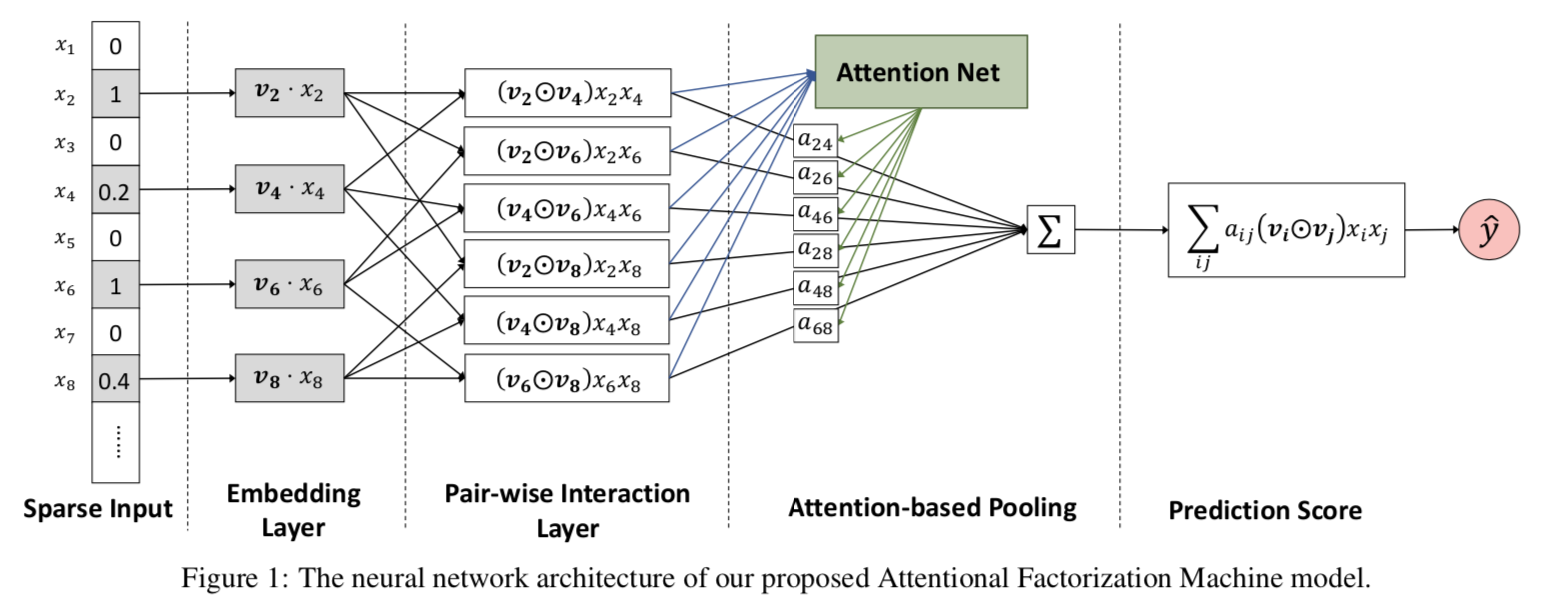
注意力部分是一个简单的全联接层，输出的是\(N(N-1)/2\)的矩阵，作为sum_pooling的权重向量，对element-wise特征交互向量进行加权求和。加权求和的向量直接连接output，不再经过全联接层。如果权重为1，那AFM和不带全联接层的NFM是一样滴。

\[\begin{align} a_{ij} &= h^T ReLU(W (v_ix_i) \odot (v_jx_j) +b) \\ a_{ij} &= \frac{exp(a_{ij})}{\sum_{ij}exp(a_{ij})}\\ \end{align} \]

AFM几个想吐槽的点

• 不带全联接层会导致高级特征表达有限，不过这个不重要啦，AFM更多还是为特征交互提供了Attention的新思路

代码实现

@tf_estimator_model
def model_fn_dense(features, labels, mode, params):
    dense_feature, sparse_feature = build_features()
    dense = tf.feature_column.input_layer(features, dense_feature) # lz linear concat of embedding
    sparse = tf.feature_column.input_layer(features, sparse_feature)

    field_size = len( dense_feature )
    embedding_size = dense_feature[0].variable_shape.as_list()[-1]
    embedding_matrix = tf.reshape( dense, [-1, field_size, embedding_size] )  # batch * field_size *emb_size

    with tf.variable_scope('Linear_part'):
        linear_output = tf.layers.dense(sparse, units=1)
        add_layer_summary( 'linear_output', linear_output )

    with tf.variable_scope('Elementwise_Interaction'):
        elementwise_list = []
        for i in range(field_size):
            for j in range(i+1, field_size):
                vi = tf.gather(embedding_matrix, indices=i, axis=1, batch_dims=0,name = 'vi') # batch * emb_size
                vj = tf.gather(embedding_matrix, indices=j, axis=1, batch_dims=0,name = 'vj')
                elementwise_list.append(tf.multiply(vi,vj)) # batch * emb_size
        elementwise_matrix = tf.stack(elementwise_list) # (N*(N-1)/2) * batch * emb_size
        elementwise_matrix = tf.transpose(elementwise_matrix, [1,0,2]) # batch * (N*(N-1)/2) * emb_size

    with tf.variable_scope('Attention_Net'):
        # 2 fully connected layer
        dense = tf.layers.dense(elementwise_matrix, units = params['attention_factor'], activation = 'relu') # batch * (N*(N-1)/2) * t
        add_layer_summary( dense.name, dense )
        attention_weight = tf.layers.dense(dense, units=1, activation = 'softmax') # batch *(N*(N-1)/2) * 1
        add_layer_summary( attention_weight.name, attention_weight)

    with tf.variable_scope('Attention_pooling'):
        interaction_output = tf.reduce_sum(tf.multiply(elementwise_matrix, attention_weight), axis=1) # batch * emb_size
        interaction_output = tf.layers.dense(interaction_output, units=1) # batch * 1

    with tf.variable_scope('output'):
        y = interaction_output + linear_output
        add_layer_summary( 'output', y )

    return y

CTR学习笔记&代码实现系列

https://github.com/DSXiangLi/CTR

CTR学习笔记&代码实现1-深度学习的前奏LR->FFM
CTR学习笔记&代码实现2-深度ctr模型 MLP->Wide&Deep
CTR学习笔记&代码实现3-深度ctr模型 FNN->PNN->DeepFM

---

资料

1. Jun Xiao, Hao Ye ,2017, Attentional Factorization Machines - Learning the Weight of Feature Interactions via Attention Networks
2. Xiangnan He, Tat-Seng Chua,2017, Neural Factorization Machines for Sparse Predictive Analytics
3. https://zhuanlan.zhihu.com/p/86181485