线性回归 - LinearRegression - 预测糖尿病 - 量化预测的质量

线性回归是分析一个变量与另外一个或多个变量（自变量）之间，关系强度的方法。

线性回归的标志，如名称所暗示的那样，即自变量与结果变量之间的关系是线性的，也就是说变量关系可以连城一条直线。

模型评估：量化预测的质量

https://scikit-learn.org/stable/modules/model_evaluation.html#model-evaluation

线性回归的 7种 预测质量方法,

1、导包,

# 导包
import numpy as np
import matplotlib.pyplot as plt
%matplotlib inline

from sklearn.linear_model import LinearRegression
import sklearn.datasets as datasets

2、加载数据集, 糖尿病数据

# 获取数据集  diabetes
data = datasets.load_diabetes()
data

{'data': array([[ 0.03807591,  0.05068012,  0.06169621, ..., -0.00259226,
          0.01990842, -0.01764613],
        [-0.00188202, -0.04464164, -0.05147406, ..., -0.03949338,
         -0.06832974, -0.09220405],
        [ 0.08529891,  0.05068012,  0.04445121, ..., -0.00259226,
          0.00286377, -0.02593034],
        ...,
        [ 0.04170844,  0.05068012, -0.01590626, ..., -0.01107952,
         -0.04687948,  0.01549073],
        [-0.04547248, -0.04464164,  0.03906215, ...,  0.02655962,
          0.04452837, -0.02593034],
        [-0.04547248, -0.04464164, -0.0730303 , ..., -0.03949338,
         -0.00421986,  0.00306441]]),
 'target': array([151.,  75., 141., 206., 135.,  97., 138.,  63., 110., 310., 101.,
         69., 179., 185., 118., 171., 166., 144.,  97., 168.,  68.,  49.,
         68., 245., 184., 202., 137.,  85., 131., 283., 129.,  59., 341.,
         87.,  65., 102., 265., 276., 252.,  90., 100.,  55.,  61.,  92.,
        259.,  53., 190., 142.,  75., 142., 155., 225.,  59., 104., 182.,
        128.,  52.,  37., 170., 170.,  61., 144.,  52., 128.,  71., 163.,
        150.,  97., 160., 178.,  48., 270., 202., 111.,  85.,  42., 170.,
        200., 252., 113., 143.,  51.,  52., 210.,  65., 141.,  55., 134.,
         42., 111.,  98., 164.,  48.,  96.,  90., 162., 150., 279.,  92.,
         83., 128., 102., 302., 198.,  95.,  53., 134., 144., 232.,  81.,
        104.,  59., 246., 297., 258., 229., 275., 281., 179., 200., 200.,
        173., 180.,  84., 121., 161.,  99., 109., 115., 268., 274., 158.,
        107.,  83., 103., 272.,  85., 280., 336., 281., 118., 317., 235.,
         60., 174., 259., 178., 128.,  96., 126., 288.,  88., 292.,  71.,
        197., 186.,  25.,  84.,  96., 195.,  53., 217., 172., 131., 214.,
         59.,  70., 220., 268., 152.,  47.,  74., 295., 101., 151., 127.,
        237., 225.,  81., 151., 107.,  64., 138., 185., 265., 101., 137.,
        143., 141.,  79., 292., 178.,  91., 116.,  86., 122.,  72., 129.,
        142.,  90., 158.,  39., 196., 222., 277.,  99., 196., 202., 155.,
         77., 191.,  70.,  73.,  49.,  65., 263., 248., 296., 214., 185.,
         78.,  93., 252., 150.,  77., 208.,  77., 108., 160.,  53., 220.,
        154., 259.,  90., 246., 124.,  67.,  72., 257., 262., 275., 177.,
         71.,  47., 187., 125.,  78.,  51., 258., 215., 303., 243.,  91.,
        150., 310., 153., 346.,  63.,  89.,  50.,  39., 103., 308., 116.,
        145.,  74.,  45., 115., 264.,  87., 202., 127., 182., 241.,  66.,
         94., 283.,  64., 102., 200., 265.,  94., 230., 181., 156., 233.,
         60., 219.,  80.,  68., 332., 248.,  84., 200.,  55.,  85.,  89.,
         31., 129.,  83., 275.,  65., 198., 236., 253., 124.,  44., 172.,
        114., 142., 109., 180., 144., 163., 147.,  97., 220., 190., 109.,
        191., 122., 230., 242., 248., 249., 192., 131., 237.,  78., 135.,
        244., 199., 270., 164.,  72.,  96., 306.,  91., 214.,  95., 216.,
        263., 178., 113., 200., 139., 139.,  88., 148.,  88., 243.,  71.,
         77., 109., 272.,  60.,  54., 221.,  90., 311., 281., 182., 321.,
         58., 262., 206., 233., 242., 123., 167.,  63., 197.,  71., 168.,
        140., 217., 121., 235., 245.,  40.,  52., 104., 132.,  88.,  69.,
        219.,  72., 201., 110.,  51., 277.,  63., 118.,  69., 273., 258.,
         43., 198., 242., 232., 175.,  93., 168., 275., 293., 281.,  72.,
        140., 189., 181., 209., 136., 261., 113., 131., 174., 257.,  55.,
         84.,  42., 146., 212., 233.,  91., 111., 152., 120.,  67., 310.,
         94., 183.,  66., 173.,  72.,  49.,  64.,  48., 178., 104., 132.,
        220.,  57.]),
 'DESCR': '.. _diabetes_dataset:\n\nDiabetes dataset\n----------------\n\nTen baseline variables, age, sex, body mass index, average blood\npressure, and six blood serum measurements were obtained for each of n =\n442 diabetes patients, as well as the response of interest, a\nquantitative measure of disease progression one year after baseline.\n\n**Data Set Characteristics:**\n\n  :Number of Instances: 442\n\n  :Number of Attributes: First 10 columns are numeric predictive values\n\n  :Target: Column 11 is a quantitative measure of disease progression one year after baseline\n\n  :Attribute Information:\n      - Age\n      - Sex\n      - Body mass index\n      - Average blood pressure\n      - S1\n      - S2\n      - S3\n      - S4\n      - S5\n      - S6\n\nNote: Each of these 10 feature variables have been mean centered and scaled by the standard deviation times `n_samples` (i.e. the sum of squares of each column totals 1).\n\nSource URL:\nhttps://www4.stat.ncsu.edu/~boos/var.select/diabetes.html\n\nFor more information see:\nBradley Efron, Trevor Hastie, Iain Johnstone and Robert Tibshirani (2004) "Least Angle Regression," Annals of Statistics (with discussion), 407-499.\n(https://web.stanford.edu/~hastie/Papers/LARS/LeastAngle_2002.pdf)',
 'feature_names': ['age',
  'sex',
  'bmi',
  'bp',
  's1',
  's2',
  's3',
  's4',
  's5',
  's6'],
 'data_filename': 'c:\\python37\\lib\\site-packages\\sklearn\\datasets\\data\\diabetes_data.csv.gz',
 'target_filename': 'c:\\python37\\lib\\site-packages\\sklearn\\datasets\\data\\diabetes_target.csv.gz'}

3、将数据分为 训练数据 和 测试数据

# 导包, 将数据分为 训练数据 和 测试数据
from sklearn.model_selection import train_test_split

X_train, X_test, y_train, y_test = train_test_split(X, y, test_size=0.1)

display (X_train.shape, y_train.shape, X_test.shape, y_test.shape)

(397, 10)
(397,)
(45, 10)
(45,)

4、建模

# 使用线性回归算法 训练数据
lr = LinearRegression()

lr.fit(X_train, y_train)

5、预测数据

# 开始预测数据
lr.predict(X_test)

array([230.00915863, 109.37448796, 135.55277842, 151.10470676,
       112.50492861,  60.06173076, 185.98893008, 154.37782567,
       226.83758259,  35.04571744,  72.66756812,  58.39584888,
       174.04109657, 236.22478163, 140.04573477, 179.59637478,
       290.40096377, 232.79655649, 127.57606558, 155.94225585,
       233.96170807, 122.18494431, 124.57198973,  97.73726963,
       261.60495587, 170.48284605, 128.85673176,  93.16011898,
       198.08756371, 179.37427503, 199.42069686, 106.91159532,
       114.42691898, 215.81999925, 200.58503886, 168.46631094,
       123.85604486, 118.02004664, 189.81321827,  80.30230583,
       108.35537981,  80.98007737, 180.839016  ,  83.22091387,
       117.70861488])

6、查看真实数据

# 查看真实的 结果值, 与上面测试结果 对比
y_test

array([246.,  69.,  40., 150., 107.,  70.,  67., 252., 236., 104.,  48.,
        77., 311., 270., 187., 200., 270., 217., 135., 144., 280., 191.,
        65., 170., 303., 138.,  42., 158., 222.,  85., 173., 129.,  68.,
       279., 248., 235., 111., 153., 101.,  77.,  72.,  42., 107., 102.,
       183.])

7、回归评价得分  (R²得分，决定系数)

回归评价7种方法,

https://scikit-learn.org/stable/modules/model_evaluation.html#r2-score-the-coefficient-of-determination

# 调用算法, 算出 评价分,   负无穷 到 1 的范围,  1为最好
lr.score(X_test, y_test)

0.5103097598041384

8、代码实现 预测评价(R²得分，决定系数)

'''
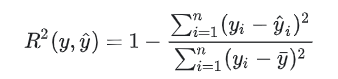
The coefficient R^2 is defined as (1 - u/v), where u is the residual
sum of squares ((y_true - y_pred) ** 2).sum() and v is the total
sum of squares ((y_true - y_true.mean()) ** 2).sum().
'''

y_pred = lr.predict(X_test).round(2)
y_true = y_test

# 代码实现  评价标准
# 真实结果: y_true
# 测试结果: y_pred

u = ((y_true - y_pred)**2).sum()
v = ((y_true - y_true.mean())**2).sum()
score = (1 - u/v)
score

0.5103097598041384