DeepLearning.ai-Week2-Residual Networks

1 - Import Packages

import numpy as np
from keras import layers
from keras.layers import Input, Add, Dense, Activation, ZeroPadding2D, BatchNormalization, Flatten, Conv2D, AveragePooling2D, MaxPooling2D, GlobalMaxPooling2D
from keras.models import Model, load_model
from keras.preprocessing import image
from keras.utils import layer_utils
from keras.utils.data_utils import get_file
from keras.applications.imagenet_utils import preprocess_input
import pydot
from IPython.display import SVG
from keras.utils.vis_utils import model_to_dot
from keras.utils import plot_model
from resnets_utils import *
from keras.initializers import glorot_uniform
import scipy.misc
from matplotlib.pyplot import imshow
%matplotlib inline

import keras.backend as K
K.set_image_data_format('channels_last')
K.set_learning_phase(1)

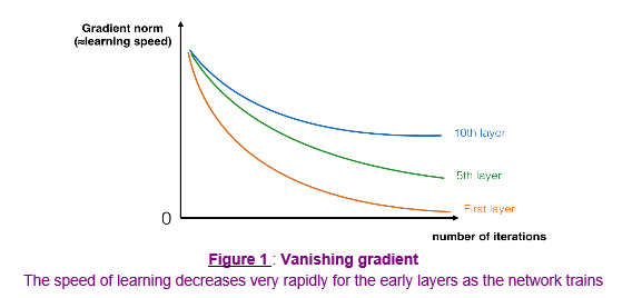
2 - The problem of very deep neural networks

　　更深的网络可以表示更复杂的函数，可以学习更多层次上的特征表示。但深层网络存在梯度消失或者梯度爆炸问题。随着训练的进行，可以看到网络前面的网络层的梯度迅速下降为0。构建$Residual Network$可以解决这个问题。

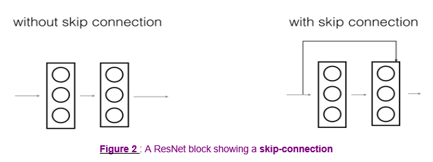
3 - Building a Residual Network

　　$Residual Network$中通过跳远连接（捷径）避免梯度消失/爆炸。跳远连接使得学习恒等函数也变得容易，所以更深的网络可以确保其效率和性能至少不低于比更浅的网络。

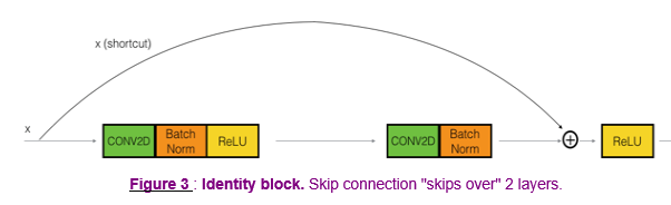
3.1 - The identity block

# GRADED FUNCTION: identity_block

def identity_block(X, f, filters, stage, block):
    """
    Implementation of the identity block as defined in Figure 3

    Arguments:
    X -- input tensor of shape (m, n_H_prev, n_W_prev, n_C_prev)
    f -- integer, specifying the shape of the middle CONV's window for the main path
    filters -- python list of integers, defining the number of filters in the CONV layers of the main path
    stage -- integer, used to name the layers, depending on their position in the network
    block -- string/character, used to name the layers, depending on their position in the network

    Returns:
    X -- output of the identity block, tensor of shape (n_H, n_W, n_C)
    """

    # defining name basis
    conv_name_base = 'res' + str(stage) + block + '_branch'
    bn_name_base = 'bn' + str(stage) + block + '_branch'

    # Retrieve Filters
    F1, F2, F3 = filters

    # Save the input value. You'll need this later to add back to the main path.
    X_shortcut = X

    # First component of main path
    X = Conv2D(filters = F1, kernel_size = (1, 1), strides = (1,1), padding = "valid", name = conv_name_base + "2a", kernel_initializer = glorot_uniform(seed=0))(X)
    X = BatchNormalization(axis = 3, name = bn_name_base + "2a")(X)
    X = Activation("relu")(X)

    ### START CODE HERE ###

    # Second component of main path (≈3 lines)
    X = Conv2D(filters = F2, kernel_size = (f, f), strides = (1, 1), padding = "same", name = conv_name_base + "2b", kernel_initializer = glorot_uniform(seed=0))(X)
    X = BatchNormalization(axis = 3, name = bn_name_base + "2b")(X)
    X = Activation("relu")(X)

    # Third component of main path (≈2 lines)
    X = Conv2D(filters = F3, kernel_size = (1, 1), strides = (1, 1), padding = "valid", name = conv_name_base + "2c", kernel_initializer = glorot_uniform(seed=0))(X)
    X = BatchNormalization(axis = 3, name = bn_name_base + "2c")(X)

    # Final step: Add shortcut value to main path, and pass it through a RELU activation (≈2 lines)
    X = Add()([X, X_shortcut])
    X = Activation("relu")(X)

    ### END CODE HERE ###

    return X

Result:
out = [ 0.94822997  0.          1.16101444  2.747859    0.          1.36677003]

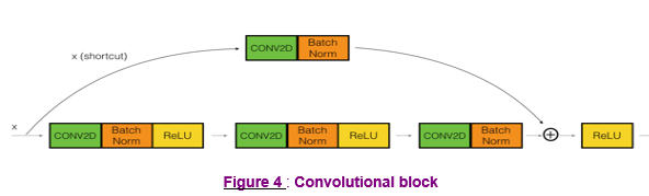
3.2 - The convolutional block

# GRADED FUNCTION: convolutional_block

def convolutional_block(X, f, filters, stage, block, s = 2):
    """
    Implementation of the convolutional block as defined in Figure 4

    Arguments:
    X -- input tensor of shape (m, n_H_prev, n_W_prev, n_C_prev)
    f -- integer, specifying the shape of the middle CONV's window for the main path
    filters -- python list of integers, defining the number of filters in the CONV layers of the main path
    stage -- integer, used to name the layers, depending on their position in the network
    block -- string/character, used to name the layers, depending on their position in the network
    s -- Integer, specifying the stride to be used

    Returns:
    X -- output of the convolutional block, tensor of shape (n_H, n_W, n_C)
    """

    # defining name basis
    conv_name_base = 'res' + str(stage) + block + '_branch'
    bn_name_base = 'bn' + str(stage) + block + '_branch'

    # Retrieve Filters
    F1, F2, F3 = filters

    # Save the input value
    X_shortcut = X

    ##### MAIN PATH #####
    # First component of main path
    X = Conv2D(F1, (1, 1), strides = (s, s), padding="valid", name = conv_name_base + "2a", kernel_initializer = glorot_uniform(seed=0))(X)
    X = BatchNormalization(axis = 3, name = bn_name_base + "2a")(X)
    X = Activation("relu")(X)

    ### START CODE HERE ###

    # Second component of main path (≈3 lines)
    X = Conv2D(F2, (f, f), strides = (1, 1), padding="same", name = conv_name_base + "2b", kernel_initializer = glorot_uniform(seed=0))(X)
    X = BatchNormalization(axis = 3, name = bn_name_base + "2b")(X)
    X = Activation("relu")(X)

    # Third component of main path (≈2 lines)
    X = Conv2D(F3, (1, 1), strides = (1, 1), padding="valid", name = conv_name_base + "2c", kernel_initializer = glorot_uniform(seed=0))(X)
    X = BatchNormalization(axis = 3, name = bn_name_base + "2c")(X)

    ##### SHORTCUT PATH #### (≈2 lines)
    X_shortcut = Conv2D(F3, (1, 1), strides = (s, s), padding="valid", name = conv_name_base + "", kernel_initializer = glorot_uniform(seed=0))(X_shortcut)
    X_shortcut = BatchNormalization(axis = 3, name = bn_name_base + "")(X_shortcut)

    # Final step: Add shortcut value to main path, and pass it through a RELU activation (≈2 lines)
    X = Add()([X, X_shortcut])
    X = Activation("relu")(X)

    ### END CODE HERE ###

    return X

tf.reset_default_graph()

with tf.Session() as test:
    np.random.seed(1)
    A_prev = tf.placeholder("float", [3, 4, 4, 6])
    X = np.random.randn(3, 4, 4, 6)
    A = convolutional_block(A_prev, f = 2, filters = [2, 4, 6], stage = 1, block = 'a')
    test.run(tf.global_variables_initializer())
    out = test.run([A], feed_dict={A_prev: X, K.learning_phase(): 0})
    print("out = " + str(out[0][1][1][0]))

Result:
out = [ 0.09018463  1.23489785  0.46822023  0.03671762  0.          0.65516603]

4 - Building your first ResNet model (50 layers)

　　"ID BLOCK"代表"Identity block"，"ID BLOCK x3"代表需要堆叠3个"Identity block"在一起。

# GRADED FUNCTION: ResNet50

def ResNet50(input_shape = (64, 64, 3), classes = 6):
    """
    Implementation of the popular ResNet50 the following architecture:
    CONV2D -> BATCHNORM -> RELU -> MAXPOOL -> CONVBLOCK -> IDBLOCK*2 -> CONVBLOCK -> IDBLOCK*3
    -> CONVBLOCK -> IDBLOCK*5 -> CONVBLOCK -> IDBLOCK*2 -> AVGPOOL -> TOPLAYER

    Arguments:
    input_shape -- shape of the images of the dataset
    classes -- integer, number of classes

    Returns:
    model -- a Model() instance in Keras
    """

    # Define the input as a tensor with shape input_shape
    X_input = Input(input_shape)

    # Zero-Padding
    X = ZeroPadding2D((3, 3))(X_input)

    # Stage 1
    X = Conv2D(64, (7, 7), strides = (2, 2), name = "conv1", kernel_initializer = glorot_uniform(seed=0))(X)
    X = BatchNormalization(axis = 3, name = "bn_conv1")(X)
    X = Activation("relu")(X)
    X = MaxPooling2D((3, 3), strides=(2, 2))(X)

    # Stage 2
    X = convolutional_block(X, f = 3, filters = [64, 64, 256], stage = 2, block="a", s = 1)
    X = identity_block(X, 3, [64, 64, 256], stage=2, block='b')
    X = identity_block(X, 3, [64, 64, 256], stage=2, block='c')

    ### START CODE HERE ###

    # Stage 3 (≈4 lines)
    X = convolutional_block(X, f = 3, filters = [128, 128, 512], stage = 3, block = "a", s = 2)
    X = identity_block(X, 3, [128, 128, 512], stage=3, block="b")
    X = identity_block(X, 3, [128, 128, 512], stage=3, block="c")
    X = identity_block(X, 3, [128, 128, 512], stage=3, block="d")

    # Stage 4 (≈6 lines)
    X = convolutional_block(X, f = 3, filters = [256, 256, 1024], stage = 4, block = "a", s = 2)
    X = identity_block(X, 3, [256, 256, 1024], stage=4, block="b")
    X = identity_block(X, 3, [256, 256, 1024], stage=4, block="c")
    X = identity_block(X, 3, [256, 256, 1024], stage=4, block="d")
    X = identity_block(X, 3, [256, 256, 1024], stage=4, block="e")
    X = identity_block(X, 3, [256, 256, 1024], stage=4, block="f")

    # Stage 5 (≈3 lines)
    X = convolutional_block(X, f = 3, filters = [512, 512, 2048], stage = 5, block = "a", s = 2)
    X = identity_block(X, 3, [512, 512, 2048], stage=5, block="b")
    X = identity_block(X, 3, [512, 512, 2048], stage=5, block="c")

    # AVGPOOL (≈1 line). Use "X = AveragePooling2D(...)(X)"
    X = AveragePooling2D(pool_size=(2, 2), name="avg_pool")(X)

    ### END CODE HERE ###

    # output layer
    X = Flatten()(X)
    X = Dense(classes, activation="softmax", name="fc" + str(classes), kernel_initializer = glorot_uniform(seed=0))(X)

    # Create model
    model = Model(inputs = X_input, outputs = X, name="ResNet50")

    return model

model = ResNet50(input_shape = (64, 64, 3), classes = 6)

model.compile(optimizer='adam', loss='categorical_crossentropy', metrics=['accuracy'])

X_train_orig, Y_train_orig, X_test_orig, Y_test_orig, classes = load_dataset()

# Normalize image vectors
X_train = X_train_orig/255.
X_test = X_test_orig/255.

# Convert training and test labels to one hot matrices
Y_train = convert_to_one_hot(Y_train_orig, 6).T
Y_test = convert_to_one_hot(Y_test_orig, 6).T

print ("number of training examples = " + str(X_train.shape[0]))
print ("number of test examples = " + str(X_test.shape[0]))
print ("X_train shape: " + str(X_train.shape))
print ("Y_train shape: " + str(Y_train.shape))
print ("X_test shape: " + str(X_test.shape))
print ("Y_test shape: " + str(Y_test.shape))

Result:
number of training examples = 1080
number of test examples = 120
X_train shape: (1080, 64, 64, 3)
Y_train shape: (1080, 6)
X_test shape: (120, 64, 64, 3)
Y_test shape: (120, 6)

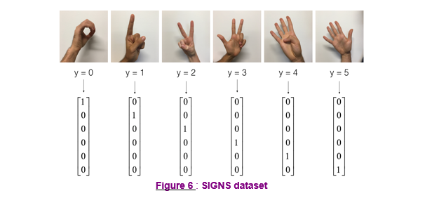
SIGNS Dataset

model.fit(X_train, Y_train, epochs = 2, batch_size = 32)

Result:

Epoch 1/2
1080/1080 [==============================] - 245s 227ms/step - loss: 3.0501 - acc: 0.2611
Epoch 2/2
1080/1080 [==============================] - 240s 223ms/step - loss: 2.3643 - acc: 0.3185

preds = model.evaluate(X_test, Y_test)
print ("Loss = " + str(preds[0]))
print ("Test Accuracy = " + str(preds[1]))

Result:
120/120 [==============================] - 8s 68ms/step
Loss = 13.4317462285
Test Accuracy = 0.166666667163

model = load_model('ResNet50.h5') 

preds = model.evaluate(X_test, Y_test)
print ("Loss = " + str(preds[0]))
print ("Test Accuracy = " + str(preds[1]))

Result: 

120/120 [==============================] - 17s 142ms/step
Loss = 0.530178316434
Test Accuracy = 0.866666662693

5 - Summary

model.summary()

Result:
（略）

plot_model(model, to_file='model.png')
SVG(model_to_dot(model).create(prog='dot', format='svg'))

Result:
（略）

6 - References

https://web.stanford.edu/class/cs230/