TensorFlow入门（一）

目录

1. TensorFlow简介
2. TensorFlow基本概念
3. Using TensorFlow
4. Optimization & Linear Regression & Logistic Regression

1. TensorFlow简介

  TensorFlow由Google的Brain Team创立，于2015年11月9日开源。

  TensorFlow中文社区网站：http://www.tensorfly.cn 。

  TensorFlow, 其含义为 Tensor + Flow, 具体说来：

• Tensor（张量）：N维数组
• Flow（流图）： 基于数据流图（Data Flow Graph）的计算

TensorFlow的特征：

1. 高度的灵活性
2. 真正的可移植性（Portability）
3. 将科研和产品联系在一起
4. 自动求微分
5. 多语言支持
6. 性能最优化

  TensorFlow Python API 在数据结构和基于多维数组的计算与NumPy有许多相似之处，其安装方式：

pip install tensorflow

  一个简单的例子："Hello world" with TensorFlow

import tensorflow as tf

h = tf.constant("Hello")
w = tf.constant(" World!")
hw = h + w
with tf.Session() as sess:
    ans = sess.run(hw)
print (ans)

2. TensorFlow基本概念

本节目录：

1. Constant
2. Tensor
3. Computation Graphs
4. Variables
5. Placeholder Variables

Constant

  TensorFlow中的常量用constant()函数构造。

Tensor

  Tensor的创建：

a = tf.constant(2)        # 标量
b = tf.constant([1,2])    # 一维向量
c = tf.constant([[1,2],
                 [3,4]])  # 二维向量

也可以指定维度（shape）以及数据类型(dtype)。比如：

a = tf.constant(np.array([1,2,3,4,5,6]), shape=(3,2),dtype=tf.int64)
a = tf.constant(np.array([[1,2,3],
                          [4,5,6]]),
                          shape=(3,2),
                          dtype=tf.float64)

Computation Graphs

Generally, the typical workflow in TensorFlow can be summarized as follows:

• Build a computational graph
• Start a new session to evaluate the graph
  1. Initialize variables
  2. Execute the operations in the compiled graph

例1：

import tensorflow as tf

a = tf.constant(5)
b = tf.constant(2)
c = tf.constant(3)

d = tf.multiply(a,b)
e = tf.add(c,b)
f = tf.subtract(d,e)

with tf.Session() as sess:
    res = sess.run(f)

print('f is %s'%res)

输出结果：

f is 5

在上述程序中，Computation Graph 示意图如下：

在TensorBoard中，Computation Graph如下：

常用的TensorFlow运算函数：

例2：使用Graph及Session

未使用Session

import tensorflow as tf

g = tf.Graph()
with g.as_default() as g:
    tf_x = tf.constant([[1., 2.],
                        [3., 4.],
                        [5.,6.]], dtype=tf.float64)
    col_sum = tf.reduce_sum(tf_x, axis=0) # 按列求和

print('tf_x:\n', tf_x)
print('col_sum:\n', col_sum)

输出结果：

tf_x:
 Tensor("Const:0", shape=(3, 2), dtype=float64)
col_sum:
 Tensor("Sum:0", shape=(2,), dtype=float64)

使用Session（获取计算结果）

import tensorflow as tf

g = tf.Graph()
with g.as_default() as g:
    tf_x = tf.constant([[1., 2.],
                        [3., 4.],
                        [5.,6.]], dtype=tf.float64)
    col_sum = tf.reduce_sum(tf_x, axis=0) # 按列求和

with tf.Session(graph=g) as sess:
    mat, csum = sess.run([tf_x, col_sum])

print('tf_x:\n', mat)
print('col_sum:\n', csum)

输出结果：

tf_x:
 [[1. 2.]
  [3. 4.]
  [5. 6.]]
col_sum:
 [ 9. 12.]

TensorFlow背后的运行原理图：

为什么要采用Computation Graphs？

• TensorFlow optimizes its computations based on the graph’s connectivity.
• Each graph has its own set of node dependencies.Being able to
  
  locate dependencies between units of our model allows us to both distribute computations across available resources and avoid performing redundant computations of irrelevant subsets, resulting in a faster and more efficient way of computing things.

Variables

  Variables are constructs in TensorFlow that allows us to store and update parameters of our models in the current session during training. To define a “variable” tensor, we use TensorFlow’s Variable() constructor. to execute a computational graph that contains variables, we must initialize all variables in the active session first (using tf.global_variables_initializer()).

例1：使用Variables

import tensorflow as tf

g = tf.Graph()
with g.as_default() as g:
    tf_x = tf.Variable([[1., 2.],
                        [3., 4.],
                        [5., 6.]], dtype=tf.float32)
    x = tf.constant(1., dtype=tf.float32)

    # add a constant to the matrix:
    tf_x = tf_x + x

with tf.Session(graph=g) as sess:
    sess.run(tf.global_variables_initializer())
    result = sess.run(tf_x)

print(result)

输出结果：

[[2. 3.]
 [4. 5.]
 [6. 7.]]

例2： 运行两遍？

运行两遍， 存在的问题：

import tensorflow as tf

g = tf.Graph()
with g.as_default() as g:
    tf_x = tf.Variable([[1., 2.],
                        [3., 4.],
                        [5., 6.]], dtype=tf.float32)
    x = tf.constant(1., dtype=tf.float32)

    # add a constant to the matrix:
    tf_x = tf_x + x

with tf.Session(graph=g) as sess:
    sess.run(tf.global_variables_initializer())
    result = sess.run(tf_x)
    result = sess.run(tf_x) # 运行两遍

print(result)

输出结果：

[[2. 3.]
 [4. 5.]
 [6. 7.]]

解决办法？ 使用tf.assign()函数。

import tensorflow as tf

g = tf.Graph()
with g.as_default() as g:
    tf_x = tf.Variable([[1., 2.],
                        [3., 4.],
                        [5., 6.]], dtype=tf.float32)
    x = tf.constant(1., dtype=tf.float32)

    # add a constant to the matrix:
    update_tf_x = tf.assign(tf_x, tf_x + x)

with tf.Session(graph=g) as sess:
    sess.run(tf.global_variables_initializer())
    result = sess.run(update_tf_x)
    result = sess.run(update_tf_x) # 运行两遍

print(result)

此时的输出结果：

[[3. 4.]
 [5. 6.]
 [7. 8.]]

Placeholder Variables

  Placeholder variables allow us to feed the computational graph with numerical values in an active session at runtime. Placeholders have an optional shape argument. If a shape is not fed or is passed as None, then the placeholder can be fed with data of any size.

例：矩阵相乘

指定行数与列数

import tensorflow as tf
import numpy as np

g = tf.Graph()
with g.as_default() as g:
    tf_x = tf.placeholder(dtype=tf.float32,shape=(3, 2))

    output = tf.matmul(tf_x, tf.transpose(tf_x)) # 矩阵乘以它的转置

with tf.Session(graph=g) as sess:
    sess.run(tf.global_variables_initializer())
    # 创建3*2矩阵
    np_ary = np.array([[3., 4.],
                       [5., 6.],
                       [7., 8.]])

    print(sess.run(output, {tf_x: np_ary}))

输出结果：

[[ 25.  39.  53.]
 [ 39.  61.  83.]
 [ 53.  83. 113.]]

指定列数

import tensorflow as tf
import numpy as np

g = tf.Graph()
with g.as_default() as g:
    tf_x = tf.placeholder(dtype=tf.float32,shape=(None, 2))

    output = tf.matmul(tf_x, tf.transpose(tf_x)) # 矩阵乘以它的转置

with tf.Session(graph=g) as sess:
    sess.run(tf.global_variables_initializer())
    # 创建3*2矩阵
    np_ary1 = np.array([[3., 4.],
                       [5., 6.],
                       [7., 8.]])

    print(sess.run(output, {tf_x: np_ary1}))

    # 创建4*2矩阵
    np_ary2 = np.array([[3., 4.],
                        [5., 6.],
                        [7., 8.],
                        [9.,10.]])

    print(sess.run(output, {tf_x: np_ary2}))

输出结果：

[[ 25.  39.  53.]
 [ 39.  61.  83.]
 [ 53.  83. 113.]]
[[ 25.  39.  53.  67.]
 [ 39.  61.  83. 105.]
 [ 53.  83. 113. 143.]
 [ 67. 105. 143. 181.]]

未指定shape

import tensorflow as tf
import numpy as np

g = tf.Graph()
with g.as_default() as g:
    tf_x = tf.placeholder(dtype=tf.float32)

    output = tf.matmul(tf_x, tf.transpose(tf_x)) # 矩阵乘以它的转置

with tf.Session(graph=g) as sess:
    sess.run(tf.global_variables_initializer())
    # 创建3*3矩阵
    np_ary1 = np.array([[3., 4., 5.],
                        [5., 6., 7.],
                        [7., 8., 9.]])

    print(sess.run(output, {tf_x: np_ary1}))

    # 创建4*2矩阵
    np_ary2 = np.array([[3., 4.],
                        [5., 6.],
                        [7., 8.],
                        [9.,10.]])

    print(sess.run(output, {tf_x: np_ary2}))

输出结果：

[[ 50.  74.  98.]
 [ 74. 110. 146.]
 [ 98. 146. 194.]]
[[ 25.  39.  53.  67.]
 [ 39.  61.  83. 105.]
 [ 53.  83. 113. 143.]
 [ 67. 105. 143. 181.]]

3. Using TensorFlow

本节目录:

• Saving and Restoring Models
• Naming TensorFlow Objects
• CPU and GPU
• Control Flow
• TensorBoard

Saving and Restoring Models

例：

Saving Models

import tensorflow as tf

g = tf.Graph()
with g.as_default() as g:

    tf_x = tf.Variable([[1., 2.],
                        [3., 4.],
                        [5., 6.]], dtype=tf.float32)
    x = tf.constant(1., dtype=tf.float32)

    update_tf_x = tf.assign(tf_x, tf_x + x)

    # initialize a Saver, which gets all variables
    # within this computation graph context
    saver = tf.train.Saver()

with tf.Session(graph=g) as sess:
    sess.run(tf.global_variables_initializer())
    result = sess.run(update_tf_x)

    # save the model
    saver.save(sess, save_path='E://flag/my-model.ckpt')

保存的文件：

The file my-model.ckpt.data-00000-of-00001 saves our main variable values, the .index file keeps track of the data structures, and the .meta file describes the structure of our computational graph that we executed.

Restoring Models:

import tensorflow as tf

g = tf.Graph()
with g.as_default() as g:

    tf_x = tf.Variable([[1., 2.],
                        [3., 4.],
                        [5., 6.]], dtype=tf.float32)
    x = tf.constant(1., dtype=tf.float32)

    update_tf_x = tf.assign(tf_x, tf_x + x)

    # initialize a Saver, which gets all variables
    # within this computation graph context
    saver = tf.train.Saver()

with tf.Session(graph=g) as sess:
    saver.restore(sess, save_path='E://flag/my-model.ckpt')
    result = sess.run(update_tf_x)
    print(result)

运行结果：

[[3. 4.]
 [5. 6.]
 [7. 8.]]

Naming TensorFlow Objects

  Each Tensor object also has an identifying name. This name is an intrinsic string name, not to be confused with the name of the variable. As with dtype, we can use the .name attribute to see the name of the object:

import tensorflow as tf

g = tf.Graph()
with g.as_default() as g:
    c1 = tf.constant(4, dtype=tf.float64, name='c')
    c2 = tf.constant(4, dtype=tf.int32, name='c')

print(c1.name)
print(c2.name)

输出：

c:0
c_1:0

Name scopes

  Sometimes when dealing with a large, complicated graph, we would like to create some node grouping to make it easier to follow and manage. For that we can hierarchically group nodes together by name. We do so by using tf.name_scope("prefix") together with the useful with clause again:

import tensorflow as tf

g = tf.Graph()
with g.as_default() as g:
    c1 = tf.constant(4, dtype=tf.float64, name='c')
    with tf.name_scope("prefix_name"):
        c2 = tf.constant(4, dtype=tf.int32, name='c')
        c3 = tf.constant(4, dtype=tf.float64, name='c')

print(c1.name)
print(c2.name)
print(c3.name)

输出：

c:0
prefix_name/c:0
prefix_name/c_1:0

CPU and GPU

  All TensorFlow operations in general, can be executed on a CPU. If you have a GPU version of TensorFlow installed, TensorFlow will automatically execute those operations that have GPU support on GPUs and use your machine’s CPU, otherwise.

Control Flow

例： if-else结构

简单的if-else语句

import tensorflow as tf

addition = True

g = tf.Graph()
with g.as_default() as g:
    x = tf.placeholder(dtype=tf.float32, shape=None)
    if addition:
        y = x + 1.
    else:
        y = x - 1.

with tf.Session(graph=g) as sess:
    result = sess.run(y, feed_dict={x: 1.})

    print('Result:\n', result)

输出：

Result:
 2.0

使用tf.cond()代替上面的if-else语句

import tensorflow as tf

g = tf.Graph()
with g.as_default() as g:
    addition = tf.placeholder(dtype=tf.bool, shape=None)
    x = tf.placeholder(dtype=tf.float32, shape=None)

    y = tf.cond(addition,
                true_fn=lambda: tf.add(x, 1.),
                false_fn=lambda: tf.subtract(x, 1.))

with tf.Session(graph=g) as sess:
    result = sess.run(y, feed_dict={addition:True,x: 1.})

    print('Result:\n', result)

输出结果：

Result:
 2.0

TensorBoard

  TensorBoard is one of the coolest features of TensorFlow, which provides us with a suite of tools to visualize our computational graphs and operations before and during runtime.

例：

import tensorflow as tf

g = tf.Graph()
with g.as_default() as g:

    tf_x = tf.Variable([[1., 2.],
                        [3., 4.],
                        [5., 6.]],
                        name='tf_x_0',
                        dtype=tf.float32)

    tf_y = tf.Variable([[7., 8.],
                        [9., 10.],
                        [11., 12.]],
                        name='tf_y_0',
                        dtype=tf.float32)

    output = tf_x + tf_y
    output = tf.matmul(tf.transpose(tf_x), output)

with tf.Session(graph=g) as sess:
    sess.run(tf.global_variables_initializer())

    # create FileWrite object that writes the logs
    file_writer = tf.summary.FileWriter(logdir='E://flag/logs/1', graph=g)
    result = sess.run(output)
    print(result)

输出结果：

[[124. 142.]
 [160. 184.]]

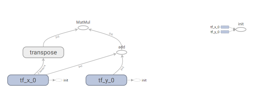
使用Tensorboard查看Computation Graph:

tensorboard --logdir E://flag/logs/1

输出结果：

C:\Users\HP>tensorboard --logdir E://flag/logs/1
TensorBoard 1.10.0 at http://DESKTOP-28K2SLS:6006 (Press CTRL+C to quit)

在浏览器中输入http://DESKTOP-28K2SLS:6006即可查看Computation Graph，截图如下：

4. Optimization & Linear Regression & Logistic Regression

Optimization Steps:

1. Defining a model
2. Defining loss function
3. Optimizer(The gradient descent)
4. Try to predict

Gradient Descent的三种形式：

描述	GD	Minth-Batches GD	SGD
单次迭代样本数	整个训练集	训练集的子集	单个样本
算法复杂度	高	一般	低
运行速度	慢	较快	快
收敛性	稳定	较稳定	不稳定
陷入局部最优点的可能性	大	较大	小

Linear Regression

1. Model

\[y = \sum\limits_{i=1}^{n}w_{i}x_{i} + b
\]

1. Loss function: MSE

\[loss = \frac{1}{2m}\sum\limits_{i=1}^{m}(y_{true} - (\sum\limits_{i=1}^{n}w_{i}x_{i}+b))^{2}
\]

1. The gradient descent optimizer(SGD)

  指定 loss function 和 learning_rate

optimizer = tf.train.GradientDescentOptimizer(learning_rate)
train = optimizer.minimize(loss)

1. predict on new sample

Linear Regression的例子：

数据集：

x_data = np.random.randn(200, 3)
w_real = [0.3, 0.5, 0.1]
b_real = -0.2
noise = np.random.randn(1, 200)*0.1
y_data = np.matmul(w_real, x_data.T) + b_real + noise

示例代码：

# -*- coding: utf-8 -*-
import numpy as np
import tensorflow as tf
from sklearn import linear_model

# 样本数据集
x_data = np.random.randn(200, 3)
w_real = [0.3, 0.5, 0.1]
b_real = -0.2
noise = np.random.randn(1, 200)*0.1
y_data = np.matmul(w_real, x_data.T) + b_real + noise

# 使用Sklearn进行一元线性回归建模
regr = linear_model.LinearRegression()

# Train the model using the data
regr.fit(x_data, y_data.transpose())

# The coefficients
w, b = regr.coef_[0], regr.intercept_
print('用Sklearn计算得到的线性回归系数:\n w:%s\tb:%s'%(w, b))

NUM_STEPS = 100                                         # 循环次数
g = tf.Graph()                                          # 创建图
wb_ = []                                                # 记录结果的列表

with g.as_default():
    x = tf.placeholder(tf.float32, shape=[None,3])       # 样本中的x值
    y_true = tf.placeholder(tf.float32, shape=None)      # 样本中的真实的y值

    with tf.name_scope('inference') as scope:
        w = tf.Variable([[0,0,0]], dtype=tf.float32, name='weights')  # w系数
        b = tf.Variable(0, dtype=tf.float32, name='bias')             # 截距b
        y_pred = tf.matmul(w, tf.transpose(x)) + b                    # y的预测值

    with tf.name_scope('loss') as scope:                              # 定义损失函数
        loss = tf.reduce_mean(tf.square(y_true-y_pred))

    with tf.name_scope('train') as scope:                             #定义optimization
        learning_rate = 0.5
        optimizer = tf.train.GradientDescentOptimizer(learning_rate)
        train = optimizer.minimize(loss)

        # Before starting, initialize the variables. We will 'run' this first.
        init = tf.global_variables_initializer()

        with tf.Session() as sess:
            sess.run(init)
            for step in range(NUM_STEPS):
                sess.run(train, {x: x_data, y_true: y_data})
            wb_.append(sess.run([w, b]))

print("用TensorFlow计算得到的线性回归系数:\n")
print(wb_)

输出结果：

用Sklearn计算得到的线性回归系数:
 w:[0.29638914 0.49420393 0.096624  ]	b:[-0.21690145]
用TensorFlow计算得到的线性回归系数:
[[array([[0.29638913, 0.49420393, 0.096624  ]], dtype=float32), -0.21690145]]

Logistic Regression

1. Model

\[\ln{(\frac{p}{1-p})} = \sum\limits_{i=1}^{n}w_{i}x_{i} + b
\]

1. Loss function: Cross Entropy (OR log loss function)

\[loss = H(p,q) = \sum\limits_{x} p(x)\log{q(x)}
\]

1. The gradient descent optimizer(SGD)

  指定 loss function 和 learning_rate

optimizer = tf.train.GradientDescentOptimizer(learning_rate)
train = optimizer.minimize(loss)

1. predict on new samples

例子：

样本数据集：

https://github.com/percent4/tensorflow_js_learning/blob/master/USA_vote.csv

Python代码：

# -*- coding: utf-8 -*-
import pandas as pd
import numpy as np
import tensorflow as tf
from sklearn.linear_model import LogisticRegression

#read data from other places, e.g. csv
#drop_list: variables that are not used
def read_data(file_path, drop_list=[]):
    dataSet = pd.read_csv(file_path,sep=',')
    for col in drop_list:
        dataSet = dataSet.drop(col,axis=1)
    return dataSet

# CSV文件存放目录
path = 'E://USA_vote.csv'
# 读取CSV文件中的数据
dataSet = read_data(path)

# 利用sklearn中的LogisticRegression模型进行建模
clf = LogisticRegression(C=1e9)
X, y = dataSet.iloc[:,0:-1], dataSet.iloc[:, -1]
clf.fit(X,y)

print('Sklearn中的逻辑回归模型计算结果：')
print(clf.coef_)
print(clf.intercept_)

y_samples = np.array(y)    # 样本中的y标签
x_samples = np.array(X)    # 样本中的x标签
samples_num, var_num = x_samples.shape

NUM_STEPS = 20000    # 总的训练次数
g = tf.Graph()
wb_ = []

# tensorflow训练模型
with g.as_default():
    x = tf.placeholder(tf.float32, shape=[None, var_num])
    y_true = tf.placeholder(tf.float32, shape=None)

    with tf.name_scope('inference') as scope:
        w = tf.Variable([[-1]*var_num], dtype=tf.float32, name='weights')
        b = tf.Variable(0, dtype=tf.float32, name='bias')
        y_pred = tf.matmul(w, tf.transpose(x)) + b

    with tf.name_scope('train') as scope:
        # labels: ture output of y, i.e. 0 and 1, logits: the model's linear prediction
        cross_entropy = tf.nn.sigmoid_cross_entropy_with_logits(labels=y_true, logits=y_pred)
        loss = tf.reduce_mean(cross_entropy)

        learning_rate = 0.5
        optimizer = tf.train.GradientDescentOptimizer(learning_rate)
        train = optimizer.minimize(loss)

        # Before starting, initialize the variables. We will 'run' this first.
        init = tf.global_variables_initializer()

        with tf.Session() as sess:
            sess.run(init)

            for step in range(NUM_STEPS):
                sess.run(train, {x: x_samples, y_true: y_samples})
                if (step % 1000 == 0):
                    # print(step, sess.run([w, b]))
                    wb_.append(sess.run([w, b]))

            print(NUM_STEPS, sess.run([w, b]))
            sess.close()

输出结果：

Sklearn中的逻辑回归模型计算结果：
[[ 0.34827234 -1.23053489 -2.74406079  6.85275877 -0.95313362 -0.47709861
   1.36435858 -1.85956934 -1.3986284   1.54663297 -3.14095297  0.78882048
   0.15680863  0.37217971 -1.44617613  0.59043785]]
[-1.56742975]
TensorFlow的计算结果：
20000 [array([[ 0.3481937 , -1.2305422 , -2.743876  ,  6.8526907 , -0.95355535,
        -0.47679362,  1.3641126 , -1.8595191 , -1.3984671 ,  1.5464842 ,
        -3.1406438 ,  0.7888262 ,  0.15678449,  0.37208068, -1.4461256 ,
         0.5904298 ]], dtype=float32), -1.56729]

Homework

  尝试着用Ridge Regression（岭回归）解决一个线性回归问题，关于Ridge Regression, 可以参考网址：https://blog.csdn.net/u012102306/article/details/52988660