YOLO v3算法介绍

图片来自https://towardsdatascience.com/yolo-v3-object-detection-with-keras-461d2cfccef6

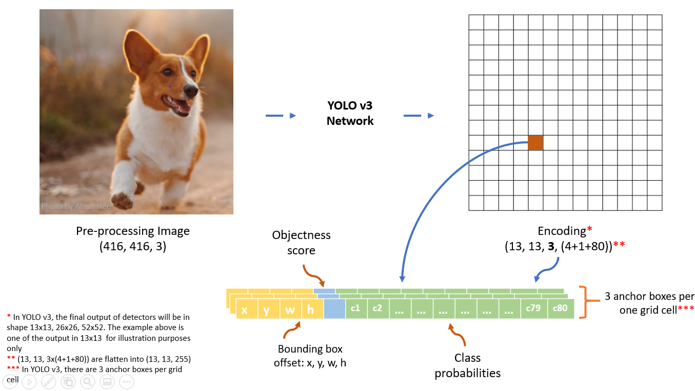
数据前处理

输入的图片维数：(416, 416, 3)

输入的图片标注：$[(x_1, y_1, x_2, y_2, class{\_}index), (x_1, y_1, x_2, y_2,class{\_}index), \ldots, (x_1, y_1, x_2, y_2,class{\_}index)]$ 表示图片中标注的所有真实box，其中$class{\_}index$代表对应的box所属的类别，$(x_1, y_1)$表示对应的box左上角的坐标值，$(x_2, y_2)$表示对应的box右下角的坐标值

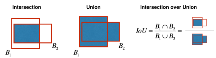
YOLO v3共有9个anchor box，每个detector中有3个anchor box。YOLO v3中anchor box的确定方法是对训练集中的所有真实box进行聚类得到的，聚类距离通过IoU来定义，IoU越大，距离越小：$$d(\text {box}, \text {centroid})=1-\operatorname{IoU}(\text {box}, \text {centroid})$$IoU的定义如下图所示：

前处理中最重要的一步就是将图片标注转化为模型的输出格式。首先要确定每个box对应哪个anchor box (与box的IoU最大的那个anchor box)，然后将box的信息写在对应的anchor box的位置。

###########以下代码仅用作说明，并未考虑性能和代码结构##########

train_output_sizes = [52, 26, 13]

label = [np.zeros((train_output_sizes[i], train_output_sizes[i], 3, 85))  for i in range(3)]

bboxes_count = np.zeros((3,))

max_bbox_per_scale = 150 #每个detector中具有的真实box的最大数量

bboxes_xywh = [np.zeros((max_bbox_per_scale, 4)) for _ in range(3)]

# YOLO v3默认的9个anchor box的width和height

anchors = [[(10,13), (16,30), (33,23)], [(30,61), (62,45), (59,119)], [(116,90), (156,198), (373,326)]]

# bboxes为一张图片中标注的所有真实box

for bbox in bboxes:

    bbox_coor = bbox[:4]

    bbox_class_ind = bbox[4]

    #onehot encode for class

    onehot = np.zeros(80, dtype=np.float)

    onehot[bbox_class_ind] = 1.0

    # 将box的坐标(x1,y1,x2,y2)转换成(xc, yc, width, height)

    bbox_xywh = np.concatenate([(bbox_coor[2:] + bbox_coor[:2]) * 0.5, bbox_coor[2:] - bbox_coor[:2]], axis=-1)

    # 找到和box有最大IoU的anchor box

    iou = []

    for anchors_detector in anchors:

        for anchor in  anchors_detector:

            intersection = min(bbox_xywh[2], anchor[0])*min(bbox_xywh[3], anchor[1])

            box_area = bbox_xywh[2]*bbox_xywh[3]

            anchor_area = anchor[0] * anchor[1]

            iou.append(intersection / (box_area + anchor_area - intersection))

    anchor_idx = np.argmax(np.array(iou))

    # 将anchor_idx转换到对应的输出位置

    best_detect = int(anchor_idx/3)

    best_anchor = int(anchor_idx % 3)

    scale = int(416/train_output_sizes[best_detect])

    xind, yind = int(bbox_xywh[0]/scale), int(bbox_xywh[1]/scale)

    label[best_detect][yind, xind, best_anchor, 0:4] = bbox_xywh

    label[best_detect][yind, xind, best_anchor, 4:5] = 1.0

    label[best_detect][yind, xind, best_anchor, 5:] = onehot

    # 存储box的信息

    bboxes_xywh[best_detect][bboxes_count[best_detect], :4] = bbox_xywh

    bboxes_count[best_detect] += 1

label_sbbox, label_mbbox, label_lbbox = label

sbboxes, mbboxes, lbboxes = bboxes_xywh

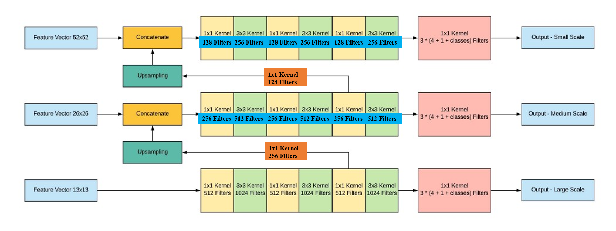
模型架构

YOLO v3的架构搭建主要分为两个部分，第一部分基于Darknet网络构建52x52, 26x26, 13x13的特征图，第二部分构建基于这三类特征图的探测器，如下图所示：

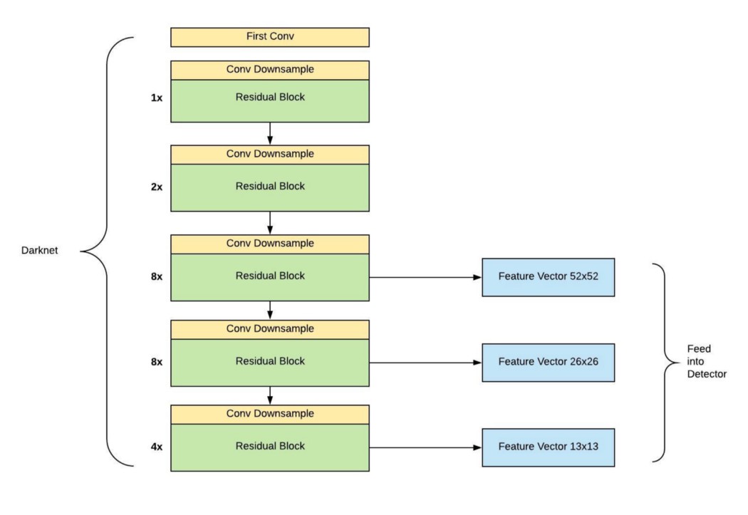
图片来自https://towardsdatascience.com/dive-really-deep-into-yolo-v3-a-beginners-guide-9e3d2666280e (对其中的错误进行了修正)

### convolutional and residual blocks

def _conv_block(inp, convs, skip=True):

    x = inp

    count = 0

    for conv in convs:

                # skip over 2 layers

        if count == (len(convs) - 2) and skip:

            skip_connection = x

        count += 1

        if conv['stride'] > 1: x = ZeroPadding2D(((1,0),(1,0)))(x) # left and top padding

        x = Conv2D(conv['filter'],

                   conv['kernel'],

                   strides=conv['stride'],

                   padding='valid' if conv['stride'] > 1 else 'same',

                   name='conv_' + str(conv['layer_idx']),

                   use_bias=False if conv['bnorm'] else True)(x)

        if conv['bnorm']: x = BatchNormalization(epsilon=0.001, name='bnorm_' + str(conv['layer_idx']))(x)

        if conv['leaky']: x = LeakyReLU(alpha=0.1, name='leaky_' + str(conv['layer_idx']))(x)

    return Add()([skip_connection, x]) if skip else x

### backbone

def make_yolov3_model():

    input_image = Input(shape=(None, None, 3)) #(416, 416,3)

    ###### Part 1 ######

    # (208, 208, 64)

    x = _conv_block(input_image, [{'filter': 32, 'kernel': 3, 'stride': 1, 'bnorm': True, 'leaky': True, 'layer_idx': 0},

                                  {'filter': 64, 'kernel': 3, 'stride': 2, 'bnorm': True, 'leaky': True, 'layer_idx': 1},

                                  {'filter': 32, 'kernel': 1, 'stride': 1, 'bnorm': True, 'leaky': True, 'layer_idx': 2},

                                  {'filter': 64, 'kernel': 3, 'stride': 1, 'bnorm': True, 'leaky': True, 'layer_idx': 3}])

    # (104, 104, 128)

    x = _conv_block(x, [{'filter': 128, 'kernel': 3, 'stride': 2, 'bnorm': True, 'leaky': True, 'layer_idx': 5},

                        {'filter':  64, 'kernel': 1, 'stride': 1, 'bnorm': True, 'leaky': True, 'layer_idx': 6},

                        {'filter': 128, 'kernel': 3, 'stride': 1, 'bnorm': True, 'leaky': True, 'layer_idx': 7}])

    # (104, 104, 128)

    x = _conv_block(x, [{'filter':  64, 'kernel': 1, 'stride': 1, 'bnorm': True, 'leaky': True, 'layer_idx': 9},

                        {'filter': 128, 'kernel': 3, 'stride': 1, 'bnorm': True, 'leaky': True, 'layer_idx': 10}])

    # (52, 52, 256)

    x = _conv_block(x, [{'filter': 256, 'kernel': 3, 'stride': 2, 'bnorm': True, 'leaky': True, 'layer_idx': 12},

                        {'filter': 128, 'kernel': 1, 'stride': 1, 'bnorm': True, 'leaky': True, 'layer_idx': 13},

                        {'filter': 256, 'kernel': 3, 'stride': 1, 'bnorm': True, 'leaky': True, 'layer_idx': 14}])

    # (52, 52, 256)

    for i in range(7):

        x = _conv_block(x, [{'filter': 128, 'kernel': 1, 'stride': 1, 'bnorm': True, 'leaky': True, 'layer_idx': 16+i*3},

                            {'filter': 256, 'kernel': 3, 'stride': 1, 'bnorm': True, 'leaky': True, 'layer_idx': 17+i*3}])

    skip_36 = x #52x52 feature map

    # (26, 26, 512)

    x = _conv_block(x, [{'filter': 512, 'kernel': 3, 'stride': 2, 'bnorm': True, 'leaky': True, 'layer_idx': 37},

                        {'filter': 256, 'kernel': 1, 'stride': 1, 'bnorm': True, 'leaky': True, 'layer_idx': 38},

                        {'filter': 512, 'kernel': 3, 'stride': 1, 'bnorm': True, 'leaky': True, 'layer_idx': 39}])

    # (26, 26, 512)

    for i in range(7):

        x = _conv_block(x, [{'filter': 256, 'kernel': 1, 'stride': 1, 'bnorm': True, 'leaky': True, 'layer_idx': 41+i*3},

                            {'filter': 512, 'kernel': 3, 'stride': 1, 'bnorm': True, 'leaky': True, 'layer_idx': 42+i*3}])

    skip_61 = x #26x26 feature map

    # (13, 13, 1024)

    x = _conv_block(x, [{'filter': 1024, 'kernel': 3, 'stride': 2, 'bnorm': True, 'leaky': True, 'layer_idx': 62},

                        {'filter':  512, 'kernel': 1, 'stride': 1, 'bnorm': True, 'leaky': True, 'layer_idx': 63},

                        {'filter': 1024, 'kernel': 3, 'stride': 1, 'bnorm': True, 'leaky': True, 'layer_idx': 64}])

    # (13, 13, 1024)

    for i in range(3):

        x = _conv_block(x, [{'filter':  512, 'kernel': 1, 'stride': 1, 'bnorm': True, 'leaky': True, 'layer_idx': 66+i*3},

                            {'filter': 1024, 'kernel': 3, 'stride': 1, 'bnorm': True, 'leaky': True, 'layer_idx': 67+i*3}]) #13x13 feature map

    ###### Part 2 ######

    # (13, 13, 512)

    x = _conv_block(x, [{'filter':  512, 'kernel': 1, 'stride': 1, 'bnorm': True, 'leaky': True, 'layer_idx': 75},

                        {'filter': 1024, 'kernel': 3, 'stride': 1, 'bnorm': True, 'leaky': True, 'layer_idx': 76},

                        {'filter':  512, 'kernel': 1, 'stride': 1, 'bnorm': True, 'leaky': True, 'layer_idx': 77},

                        {'filter': 1024, 'kernel': 3, 'stride': 1, 'bnorm': True, 'leaky': True, 'layer_idx': 78},

                        {'filter':  512, 'kernel': 1, 'stride': 1, 'bnorm': True, 'leaky': True, 'layer_idx': 79}], skip=False)

    # (13, 13, 255)

    yolo_82 = _conv_block(x, [{'filter': 1024, 'kernel': 3, 'stride': 1, 'bnorm': True,  'leaky': True,  'layer_idx': 80},

                              {'filter':  255, 'kernel': 1, 'stride': 1, 'bnorm': False, 'leaky': False, 'layer_idx': 81}], skip=False) #13x13 detector

    # concatenate with 26x26 feature map, (26, 26, 256+512)

    x = _conv_block(x, [{'filter': 256, 'kernel': 1, 'stride': 1, 'bnorm': True, 'leaky': True, 'layer_idx': 84}], skip=False)

    x = UpSampling2D(2)(x)

    x = Concatenate()([x, skip_61])

    # (26, 26, 256)

    x = _conv_block(x, [{'filter': 256, 'kernel': 1, 'stride': 1, 'bnorm': True, 'leaky': True, 'layer_idx': 87},

                        {'filter': 512, 'kernel': 3, 'stride': 1, 'bnorm': True, 'leaky': True, 'layer_idx': 88},

                        {'filter': 256, 'kernel': 1, 'stride': 1, 'bnorm': True, 'leaky': True, 'layer_idx': 89},

                        {'filter': 512, 'kernel': 3, 'stride': 1, 'bnorm': True, 'leaky': True, 'layer_idx': 90},

                        {'filter': 256, 'kernel': 1, 'stride': 1, 'bnorm': True, 'leaky': True, 'layer_idx': 91}], skip=False)

    # (26, 26, 255)

    yolo_94 = _conv_block(x, [{'filter': 512, 'kernel': 3, 'stride': 1, 'bnorm': True,  'leaky': True,  'layer_idx': 92},

                              {'filter': 255, 'kernel': 1, 'stride': 1, 'bnorm': False, 'leaky': False, 'layer_idx': 93}], skip=False) #26x26 detector

    # concatenate with 52x52 feature map, (52, 52, 128+256)

    x = _conv_block(x, [{'filter': 128, 'kernel': 1, 'stride': 1, 'bnorm': True, 'leaky': True,   'layer_idx': 96}], skip=False)

    x = UpSampling2D(2)(x)

    x = Concatenate()([x, skip_36])

    # (52, 52, 255)

    yolo_106 = _conv_block(x, [{'filter': 128, 'kernel': 1, 'stride': 1, 'bnorm': True,  'leaky': True,  'layer_idx': 99},

                               {'filter': 256, 'kernel': 3, 'stride': 1, 'bnorm': True,  'leaky': True,  'layer_idx': 100},

                               {'filter': 128, 'kernel': 1, 'stride': 1, 'bnorm': True,  'leaky': True,  'layer_idx': 101},

                               {'filter': 256, 'kernel': 3, 'stride': 1, 'bnorm': True,  'leaky': True,  'layer_idx': 102},

                               {'filter': 128, 'kernel': 1, 'stride': 1, 'bnorm': True,  'leaky': True,  'layer_idx': 103},

                               {'filter': 256, 'kernel': 3, 'stride': 1, 'bnorm': True,  'leaky': True,  'layer_idx': 104},

                               {'filter': 255, 'kernel': 1, 'stride': 1, 'bnorm': False, 'leaky': False, 'layer_idx': 105}], skip=False) #52x52 detector

    model = Model(input_image, [yolo_82, yolo_94, yolo_106])

    return model

损失函数

YOLO v3中的损失函数有许多不同的变种，这里选取一种比较经典的进行介绍。损失函数可以分解为边框损失、目标损失以及分类损失这三项之和，下面对这三项逐一进行介绍。

边框损失：原始论文中使用MSE(均方误差)作为边框的损失函数，但是不同质量的预测结果，利用MSE有时候并不能区分开来。使用IoU更能体现回归框的质量，并且具有尺度不变性，但是IoU仅能描述两个边框重叠的面积，不能描述两个边框重叠的形式；并且若两个边框完全不相交，则IoU为0，不适合继续进行梯度优化。GIoU (Generalized IoU)继承了IoU的优点，并且一定程度上解决了IoU存在的问题：$$G I o U=I o U-\frac{|C \backslash(B_1 \cup B_2)|}{|C|}$$其中$C$为包含$B_1$与$B_2$的最小封闭形状。边框损失可表示为$1-G I o U$，下面以13x13这一检测器为例来计算边框损失，总的边框损失为三个检测器的损失之和。

要计算边框损失，首先要对YOLO v3的网络输出进行转换，假设网络输出的边框信息为$(t_x,t_y,t_w,t_h)$，其中$(t_x,t_y)$为边框中心点信息，$(t_w,t_h)$为边框的宽度和高度信息，转换公式如下所示：$$b_x=sigmoid(t_x)+c_x;\text{ }b_y=sigmoid(t_y)+c_y;\text{ }b_w=p_wexp(t_w);\text{ }b_h=p_hexp(t_h)$$其中$(c_x,c_y)$表示$(t_x,t_y)$所在网格的左上角那个点的坐标位置，$(p_w,p_h)$表示边框对应的anchor box的宽度和高度。

output_size = 13

anchors = np.array([[116,90], [156,198], [373,326]]) #anchor boxes in 13x13 detector, 参见数据前处理代码部分

# yolo_82_batch: 13x13 detector output, (batch_size, 13, 13, 255), yolo_82的计算参见模型架构代码部分

conv_output = tf.reshape(yolo_82_batch, (batch_size, output_size, output_size, 3, 85))  #(batch_size, 13, 13, 3, 85)

t_xy, t_wh, objectness, classes = tf.split(conv_output, (2, 2, 1, 80), axis=-1) #t_xy:(batch_size, 13, 13, 3, 2); t_wh:(batch_size, 13, 13, 3, 2)

c_xy = tf.meshgrid(tf.range(output_size), tf.range(output_size)) #a list of two (13,13) arrays

c_xy = tf.stack(c_xy, axis=-1) #(13,13,2)

c_xy = tf.tile(c_xy[tf.newaxis, :, :, tf.newaxis, :], [batch_size, 1, 1, 3, 1]) #(batch_size,13,13,3,2)

scale = int(416/output_size)

b_xy = (tf.sigmoid(t_xy) + c_xy) * scale #(batch_size,13,13,3,2)

b_wh = tf.exp(t_wh) * anchors #(batch_size,13,13,3,2)

b_xywh = tf.concat([b_xy, b_wh], axis=-1) #(batch_size,13,13,3,4)

接下来计算网络输出的边框与真实边框的GIoU，进而得到边框损失：

def bbox_giou(boxes1, boxes2):

    # transform from (xc, yc, w, h) to (xmin, ymin, xmax, ymax)

    boxes1 = tf.concat([boxes1[..., :2] - boxes1[..., 2:] * 0.5,

                        boxes1[..., :2] + boxes1[..., 2:] * 0.5], axis=-1)

    boxes2 = tf.concat([boxes2[..., :2] - boxes2[..., 2:] * 0.5,

                        boxes2[..., :2] + boxes2[..., 2:] * 0.5], axis=-1)

    # two box aeras

    boxes1_area = (boxes1[..., 2] - boxes1[..., 0]) * (boxes1[..., 3] - boxes1[..., 1])

    boxes2_area = (boxes2[..., 2] - boxes2[..., 0]) * (boxes2[..., 3] - boxes2[..., 1])

    # intersection area

    left_up = tf.maximum(boxes1[..., :2], boxes2[..., :2])

    right_down = tf.minimum(boxes1[..., 2:], boxes2[..., 2:])

    inter_section = tf.maximum(right_down - left_up, 0.0)

    inter_area = inter_section[..., 0] * inter_section[..., 1]

    # compute iou

    union_area = boxes1_area + boxes2_area - inter_area

    iou = inter_area / union_area

    # enclosed area

    enclose_left_up = tf.minimum(boxes1[..., :2], boxes2[..., :2])

    enclose_right_down = tf.maximum(boxes1[..., 2:], boxes2[..., 2:])

    enclose = tf.maximum(enclose_right_down - enclose_left_up, 0.0)

    enclose_area = enclose[..., 0] * enclose[..., 1]

    # compute giou

    giou = iou - 1.0 * (enclose_area - union_area) / enclose_area

    return giou

### label_lbbox_batch: ground truth boxes in 13x13 detector, (batch_size, 13, 13, 3, 85), label_lbbox的计算参见数据前处理代码部分

label_xywh    = label_lbbox_batch[:, :, :, :, 0:4] #ground truth box (xc, yc, w, h)

respond_bbox  = label_lbbox_batch[:, :, :, :, 4:5] #对应的anchor box内是否有真实对象存在，为1则计算边框损失，为0则忽略

giou = tf.expand_dims(bbox_giou(b_xywh, label_xywh), axis=-1) #(batch_size, 13, 13, 3, 1)

input_size = tf.cast(416, tf.float32)

bbox_loss_scale = 2.0 - 1.0 * label_xywh[:, :, :, :, 2:3] * label_xywh[:, :, :, :, 3:4] / (input_size ** 2) #边框损失的权重，对应的ground truth box的面积越大，对错误的容忍率越高，赋予的权重越小

giou_loss = respond_bbox * bbox_loss_scale * (1- giou) #giou loss, (batch_size, 13, 13, 3, 1)

目标损失：仍以13x13这一检测器为例来计算，目标损失实际上是一个不平衡二分类问题，因为一般来说检测器的13x13x3个anchor box内真实对象（正样本）的数量要远小于没有真实对象（负样本）的数量。采用Focal Loss来处理这一问题，Focal Loss对难分类的样本采用较大的权重，对易分类的样本采用较小的权重：$$F L(p)=\left\{\begin{aligned}-(1-p)^{\gamma} \log (p), & \text { positive samples } \\ -p^{\gamma} \log (1-p), & \text { negative samples }\end{aligned}\right.$$Focal Loss还有另外一种公式，即在上述基础上引入类别权重$\alpha$：$$F L(p)=\left\{\begin{aligned}-\alpha(1-p)^{\gamma} \log (p), & \text { positive samples} \\ -(1-\alpha) p^{\gamma} \log (1-p), & \text { negative samples }\end{aligned}\right.$$本文采用第一种公式，并将$\gamma$设为2。另外在目标损失的计算过程中对负样本的定义进行了一定修改，如果一个anchor box内没有真实对象，但它预测的边框和对应的探测器上的某个真实边框有较大的IoU，那么就不把它作为负样本，从而在损失计算过程中忽略它，这也在一定程度上减少了负样本的数量。

### lbboxes_batch: 13x13探测器上存在的所有ground truth box的(xc,yc,w,h)信息, (batch_size, max_bbox_per_scale, 4), lbboxes的计算参见数据前处理代码部分

### label_lbbox_batch: ground truth boxes in 13x13 detector, (batch_size, 13, 13, 3, 85), label_lbbox的计算参见数据前处理代码部分

### objectness：预测的对象真实度, (batch_size, 13, 13, 3, 1), 参见边框损失中的输出转换代码部分

### b_xywh: 预测的边框信息，(batch_size, 13, 13, 3, 4), 参见边框损失中的输出转换代码部分

respond_bbox = label_lbbox_batch[:, :, :, :, 4:5] #对应的anchor box内是否有真实对象存在，为1则为正样本，为0则为负样本

### 减少进行计算的负样本的数量 ###

### 1. 计算预测的box与所有真实box的IoU ###

boxes1 = tf.tile(lbboxes_batch[:, tf.newaxis, tf.newaxis, tf.newaxis, :, :], [1, 13, 13, 3, 1, 1]) #(batch_size, 13, 13, 3, max_bbox_per_scale, 4)

boxes2 = tf.tile(b_xywh[:, :, :, :, tf.newaxis, :], [1, 1, 1, 1, max_bbox_per_scale, 1]) #(batch_size, 13, 13, 3, max_bbox_per_scale, 4)

boxes1_area = boxes1[..., 2] * boxes1[..., 3]

boxes2_area = boxes2[..., 2] * boxes2[..., 3]

# (xc, yc, w, h)->(xmin, ymin, xmax, ymax)

boxes1 = tf.concat([boxes1[..., :2] - boxes1[..., 2:] * 0.5, boxes1[..., :2] + boxes1[..., 2:] * 0.5], axis=-1)

boxes2 = tf.concat([boxes2[..., :2] - boxes2[..., 2:] * 0.5, boxes2[..., :2] + boxes2[..., 2:] * 0.5], axis=-1)

# compute IoU

left_up = tf.maximum(boxes1[..., :2], boxes2[..., :2])

right_down = tf.minimum(boxes1[..., 2:], boxes2[..., 2:])

inter_section = tf.maximum(right_down - left_up, 0.0)

inter_area = inter_section[..., 0] * inter_section[..., 1]

union_area = boxes1_area + boxes2_area - inter_area

iou = 1.0 * inter_area / union_area #(batch_size, 13, 13, 3, max_bbox_per_scale)

### 2. 寻找最大的IoU，若该值大于给定的临界值，则在损失计算中忽略该样本###

max_iou = tf.expand_dims(tf.reduce_max(iou, axis=-1), axis=-1) #(batch_size, 13, 13, 3, 1)

IOU_LOSS_THRESH = 0.5

respond_bgd = (1.0 - respond_bbox) * tf.cast( max_iou < IOU_LOSS_THRESH, tf.float32) #(batch_size, 13, 13, 3, 1)

###########################

pred_conf  = tf.sigmoid(objectness) #预测为真实对象的概率

conf_focal = tf.pow(respond_bbox - pred_conf, 2) #gamma=2

focal_loss_p = conf_focal * respond_bbox * tf.nn.sigmoid_cross_entropy_with_logits(labels=respond_bbox, logits=objectness) #正样本损失

focal_loss_n = conf_focal * respond_bgd * tf.nn.sigmoid_cross_entropy_with_logits(labels=respond_bbox, logits=objectness) #负样本损失

focal_loss = focal_loss_p + focal_loss_n #(batch_size, 13, 13, 3, 1)

分类损失：仍以13x13这一检测器为例来计算，使用交叉熵损失函数，值得注意的是在YOLO v3的类别预测中使用sigmoid作为激活函数代替之前的softmax，主要是因为不同的类别不一定是互斥的，一个对象可能会同时属于多个类别。

### label_lbbox_batch: ground truth boxes in 13x13 detector, (batch_size, 13, 13, 3, 85), label_lbbox的计算参见数据前处理代码部分

### classes: 预测对象所属的类别，(batch_size, 13, 13, 3, 80), 参见边框损失中的输出转换代码部分

respond_bbox  = label_lbbox_batch[:, :, :, :, 4:5] #对应的anchor box内是否有真实对象存在，为1则计算分类损失，为0则忽略

labels_onehot = label_lbbox_batch[:, :, :, :, 5:] #对象所属的真实类别

classes_prob  = tf.sigmoid(classes) #预测属于每个类别的概率

ce_loss = respond_bbox * tf.nn.sigmoid_cross_entropy_with_logits(labels=labels_onehot, logits=classes) #cross entropy loss, (batch_size, 13, 13, 3, 80)

综合上述的三类损失，可以计算出在13x13探测器上的总损失，其余两个探测器 (26x26, 52x52) 上的损失可采取同样的方法计算，三个探测器的总损失为：

giou_loss_13 = tf.reduce_mean(tf.reduce_sum(giou_loss, axis=[1,2,3,4]))

focal_loss_13 = tf.reduce_mean(tf.reduce_sum(focal_loss, axis=[1,2,3,4]))

ce_loss_13 = tf.reduce_mean(tf.reduce_sum(ce_loss, axis=[1,2,3,4]))

total_loss_13 = giou_loss_13 + focal_loss_13 + ce_loss_13

# total loss

total_loss = total_loss_13 + total_loss_26 + total_loss_52

模型预测

同损失函数这一部分中的介绍，首先将网络输出的格式进行转换：

### 仍以13x13检测器为例, 输入的待预测图片的维数为(1, 416, 416, 3)

### b_xywh, pred_conf, classes_prob的计算参见损失函数代码部分

output_13 = tf.concat([b_xywh, pred_conf, classes_prob], axis=-1) #(batch_size, 13, 13, 3, 85)，此时的batch_size为1

### 同样的方式可以计算出output_26 (26x26检测器), output_52 (52x52检测器)

### output_26: (1, 26, 26, 3, 85); output_52: (1, 52, 52, 3, 85)

pred_bbox = [tf.reshape(x, (-1, tf.shape(x)[-1])) for x in (output_13, output_26, output_52)] #[(13*13*3, 85), (26*26*3, 85), (52*52*3, 85)]

pred_bbox = tf.concat(pred_bbox, axis=0) #预测得到的所有box的信息, (13*13*3+26*26*3+52*52*3, 85)

接下来删除得分较低的预测box，得分通过box内为真实对象的概率乘以最大的类别概率进行确定

score_threshold = 0.5

pred_xywh = pred_bbox[:, 0:4]

# (xc, yc, w, h) --> (xmin, ymin, xmax, ymax) for computing IoU

pred_coor = np.concatenate([pred_xywh[:, :2] - pred_xywh[:, 2:] * 0.5, pred_xywh[:, :2] + pred_xywh[:, 2:] * 0.5], axis=-1)

# compute box score

pred_conf = pred_bbox[:, 4]

pred_prob = pred_bbox[:, 5:]

classes = np.argmax(pred_prob, axis=-1) #每个box预测的对应最大概率的类别

scores = pred_conf * np.max(pred_prob, axis=-1)

# discard boxes with low scores

mask = scores > score_threshold

coors, scores, classes = pred_coor[mask], scores[mask], classes[mask]

filter_boxes = np.concatenate([coors, scores[:, np.newaxis], classes[:, np.newaxis]], axis=-1) #(number of remaining boxes, 6)

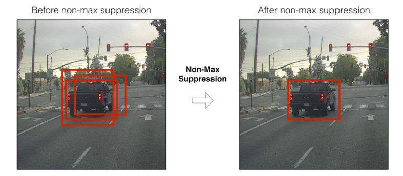
对剩余的预测box进行Non-Maximum Suppression (NMS)，NMS的主要目的是去除预测类别相同但是重叠度比较大的box:

iou_threshold = 0.5

classes_in_img = list(set(filter_boxes[:, 5])) #图片上的所有预测类别

best_bboxes = [] #最终剩余的box

for cls in classes_in_img:

    cls_mask = (filter_boxes[:, 5] == cls)

    cls_bboxes = filter_boxes[cls_mask] #预测为同一类别的所有box

    while len(cls_bboxes) > 0:

        max_ind = np.argmax(cls_bboxes[:, 4])

        best_bbox = cls_bboxes[max_ind] #剩余box中得分最高的box

        best_bboxes.append(best_bbox)

        ### 计算得分最高的box与剩余box的IoU ###

        cls_bboxes = np.concatenate([cls_bboxes[: max_ind], cls_bboxes[max_ind + 1:]], axis=0) #剩余box (不包括得分最高的box)

        best_bbox_xy = best_bbox[np.newaxis, :4]

        cls_bboxes_xy = cls_bboxes[:, :4]

        ### IoU

        best_bbox_area = (best_bbox_xy[:, 2] - best_bbox_xy[:, 0]) * (best_bbox_xy[:, 3] - best_bbox_xy[:, 1])

        cls_bboxes_area = (cls_bboxes_xy[:, 2] - cls_bboxes_xy[:, 0]) * (cls_bboxes_xy[:, 3] - cls_bboxes_xy[:, 1])

        left_up = np.maximum(best_bbox_xy[:, :2], cls_bboxes_xy[:, :2])

        right_down = np.minimum(best_bbox_xy[:, 2:], cls_bboxes_xy[:, 2:])

        inter_section = np.maximum(right_down - left_up, 0.0)

        inter_area = inter_section[:, 0] * inter_section[:, 1]

        union_area = cls_bboxes_area + best_bbox_area - inter_area

        ious = 1.0 * inter_area / union_area

        ### 删除与得分最高的box的IoU较大的box ###

        iou_mask = ious < iou_threshold

        cls_bboxes = cls_bboxes[iou_mask]

参考资料

本文主要针对YOLO v3的细节进行了总结，对目标检测以及YOLO系列的基础概念并未详细说明，这部分可以参考Coursera上深度学习专项课程中的Convolutional Neural Networks
本文的代码部分仅是为了用于说明，并没有进行系统地设计和优化，YOLO v3的代码可以参考以下链接
- https://github.com/YunYang1994/TensorFlow2.0-Examples/tree/master/4-Object_Detection/YOLOV3
- https://github.com/experiencor/keras-yolo3
其它资料