Jun

Contents

• 数据来源
• 代码演示
• 讨论
  

  一.数据来源

为了节省时间，我直接用了官方所给的数据，分别是雄性和雌性小鼠的肝脏芯片数据

Female Data

Male Data

二.代码演示

数据输入

    library(WGCNA)
    femData<-read.csv("LiverFemale3600.csv")
    dim(femData)
    names(femData)
    datExpr0 = as.data.frame(t(femData[, -c(1:8)]))
    names(datExpr0) = femData$substanceBXH
    rownames(datExpr0) = names(femData)[-c(1:8)]
    gsg = goodSamplesGenes(datExpr0, verbose = 3)##剔除不合格的基因

    Step2 样本聚类
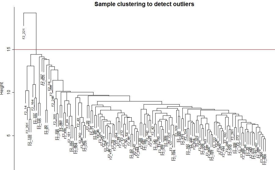
    sampleTree = hclust(dist(datExpr0), method = "average")##样本聚类，可以反映样本的重    复性，也可以看出离群样本有哪些
    sizeGrWindow(12,9)
    par(cex = 0.6)
    (mar = c(0,4,2,0))
    plot(sampleTree, main = "Sample clustering to detect outliers", sub="", xlab="",     cex.lab = 1.5,
    cex.axis = 1.5, cex.main = 2)

    abline(h = 15, col = "red")
    clust = cutreeStatic(sampleTree, cutHeight = 15, minSize = 10)
    table(clust)
    keepSamples = (clust==1)
    datExpr = datExpr0[keepSamples, ]
    nGenes = ncol(datExpr)
    nSamples = nrow(datExpr)

    Step3 阈值计算
    powers = c(c(1:10), seq(from = 12, to=20, by=2))##计算软阈值
    sft = pickSoftThreshold(datExpr, powerVector = powers, verbose = 5)##sft返回的是一个列表
    sizeGrWindow(9, 5)
    par(mfrow = c(1,2))
    cex1 = 0.9
    plot(sft$fitIndices[,1], -sign(sft$fitIndices[,3])*sft$fitIndices[,2],
    xlab="Soft Threshold (power)",ylab="Scale Free Topology Model Fit,signed R^2",type="n",
    main = paste("Scale independence"))
    text(sft$fitIndices[,1], -sign(sft$fitIndices[,3])*sft$fitIndices[,2],
    labels=powers,cex=cex1,col="red")
    abline(h=0.90,col="red")
    plot(sft$fitIndices[,1], sft$fitIndices[,5],
    xlab="Soft Threshold (power)",ylab="Mean Connectivity", type="n",
    main = paste("Mean connectivity"))
    text(sft$fitIndices[,1], sft$fitIndices[,5], labels=powers, cex=cex1,col="red")

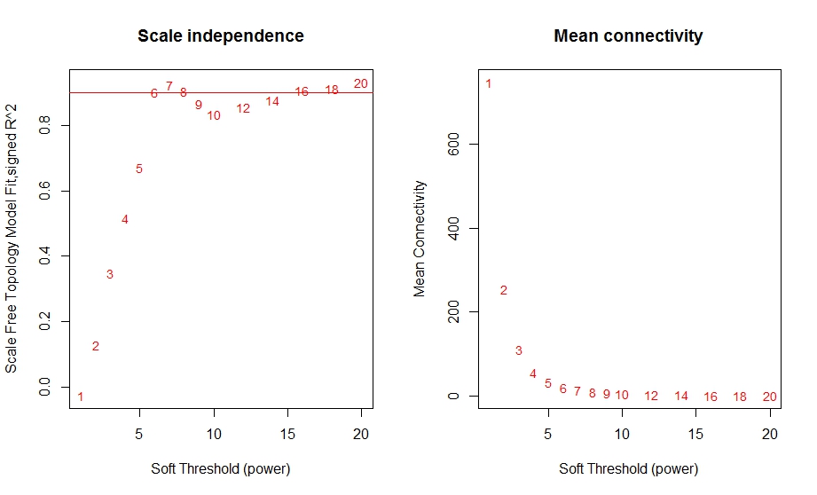
经过上面代码的运行，得出了软阈值的结果。从左图中可以看到，当阈值达到6时，整个网络就已经靠近无尺度网络的分布了，R方也达到了0.95左右的水平。sft这个列表当中的powerEstimate代表的便是最佳阈值。右图代表的是整个网络中，随着阈值的变化，整个网络中节点(Gene)间的连接度均值，符合幂率分布。

    Step4 网络构建
    net = blockwiseModules(datExpr, power = sft$powerEstimate,
                       TOMType = "unsigned", minModuleSize = 30,
                       reassignThreshold = 0, mergeCutHeight = 0.25,
                       numericLabels = TRUE, pamRespectsDendro = FALSE,
                       saveTOMs = TRUE,
                       saveTOMFileBase = "femaleMouseTOM", verbose = 3)##一步法构建网络

    Step5 模块上色
    sizeGrWindow(12, 9)
    mergedColors = labels2colors(net$colors)
    plotDendroAndColors(net$dendrograms[[1]], mergedColors[net$blockGenes[[1]]],
                    "Module colors",
                    dendroLabels = FALSE, hang = 0.03,
                    addGuide = TRUE, guideHang = 0.05)
    moduleLabels = net$colors
    moduleColors = labels2colors(net$colors)##模块上色
    = net$MEs;
    geneTree = net$dendrograms[[1]]
    table(moduleColors)##查看模块对应的颜色及模块内的基因

    moduleColors
       black         blue        brown         cyan        green  greenyellow         grey       grey60
         208          456          415           79          314          102           99           47
   lightcyan   lightgreen      magenta midnightblue         pink       purple          red       salmon
          47           34          123           79          149          123          212           94
         tan    turquoise       yellow
         100          595          324

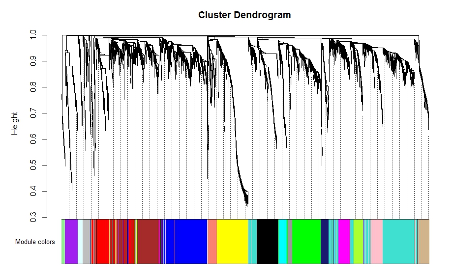
在众多模块当中，grey模块里的基因代表无法被归类到任何一个模块里的基因。同时，WGCNA也可以将距离较近的模块合并.

     Step6 联系表型信息
    traitData = read.csv("ClinicalTraits.csv")##引入表型信息相关数据
    dim(traitData)
    names(traitData)
    allTraits = traitData[, -c(31, 16)]##选取部分信息
    allTraits = allTraits[, c(2, 11:36) ]
    dim(allTraits)
    names(allTraits)

    femaleSamples = rownames( 大专栏  JundatExpr);
    traitRows = match(femaleSamples, allTraits$Mice)
    datTraits = allTraits[traitRows, -1]
    rownames(datTraits) = allTraits[traitRows, 1]

    collectGarbage()

    nGenes = ncol(datExpr)
    nSamples = nrow(datExpr)
    MEs0 = moduleEigengenes(datExpr, moduleColors)$eigengenes
    MEs = orderMEs(MEs0)
    moduleTraitCor = cor(MEs, datTraits, use = "p")#计算模块和表型信息的相关系数
    moduleTraitPvalue = corPvalueStudent(moduleTraitCor, nSamples)

    sizeGrWindow(10,6)
    textMatrix =  paste(signif(moduleTraitCor, 2), "n(",
                  signif(moduleTraitPvalue, 1), ")", sep = "")
    (textMatrix) = dim(moduleTraitCor)
    par(mar = c(6, 8.5, 3, 3))
    #绘制表型和模块的相关性热图
    labeledHeatmap(Matrix = moduleTraitCor,
               xLabels = names(datTraits),
               yLabels = names(MEs),
               ySymbols = names(MEs),
               colorLabels = FALSE,
               colors = greenWhiteRed(50),
               textMatrix = textMatrix,
               setStdMargins = FALSE,
               cex.text = 0.5,
               zlim = c(-1,1),
               main = paste("Module-trait relationships"))

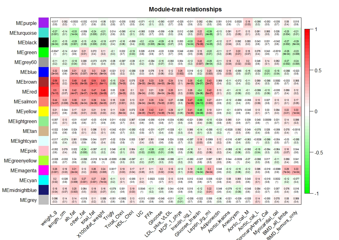
通过模块与表型相关性热图中可以看到：brown、red模块与weight有较高的相关性。研究者可以根据上述信息研究与目标表型相关联的模块，也可以研究感兴趣的模块。

比较值得注意的是，即使算出了模块与表型的相关性，一个模块里也往往存在着比较多的基因。那么具体哪些基因值得我们去做后续的分析，还需要对模块进行更深一步的细化研究。

    Step7 GSvsMM
    weight = as.data.frame(datTraits$weight_g)
    names(weight) = "weight"
    modNames = substring(names(MEs), 3)
    geneModuleMembership = as.data.frame(cor(datExpr, MEs, use = "p"))##计算模块MM值与基因间的相关系数，datExpr为表达量
    MMPvalue = as.data.frame(corPvalueStudent(as.matrix(geneModuleMembership), nSamples))

    names(geneModuleMembership) = paste("MM", modNames, sep="")
    names(MMPvalue) = paste("p.MM", modNames, sep="")

    geneTraitSignificance = as.data.frame(cor(datExpr, weight, use = "p"))##计算表型weight与基因间的相关系数
    GSPvalue = as.data.frame(corPvalueStudent(as.matrix(geneTraitSignificance), nSamples))

    names(geneTraitSignificance) = paste("GS.", names(weight), sep="")
    names(GSPvalue) = paste("p.GS.", names(weight), sep="")

在WGCNA中，定义了GS值和MM值。那么上面的代码可以简单的理解为：分别计算，ME值与基因间的相关系数，以及计算基因和表型间的相关系数。通过计算，那些不仅与模块高度相关的而且与表型也高度相关的基因就非常值得研究了。与模块高度相关的基因，往往也在这个模块中具有重要的地位或者说具有中心要素。

     module = "brown"
    column = match(module, modNames)
    moduleGenes = moduleColors==module

    sizeGrWindow(7, 7);
    par(mfrow = c(1,1));
    verboseScatterplot(abs(geneModuleMembership[moduleGenes, column]),
                   abs(geneTraitSignificance[moduleGenes, 1]),
                   xlab = paste("Module Membership in", module, "module"),
                   ylab = "Gene significance for body weight",
                   main = paste("Module membership vs. gene significancen"),
                   cex.main = 1.2, cex.lab = 1.2, cex.axis = 1.2, col = module)

    Step8 导出指定模块基因名
    module = "brown"
    probes = names(datExpr)
    inModule = (moduleColors==module)
    modProbes = probes[inModule]
    table(modProbes)

    Step9 导出模块网络
    TOM = TOMsimilarityFromExpr(datExpr, power = 6)#这一步非常消耗内存
    module = "brown"
    probes = names(datExpr)
    inModule = (moduleColors==module)
    modProbes = probes[inModule]
    modTOM = TOM[inModule, inModule]
    dimnames(modTOM) = list(modProbes, modProbes)

    #visant格式导出
    vis = exportNetworkToVisANT(modTOM,
      file = paste("VisANTInput-", module, ".txt", sep=""),
      weighted = TRUE,
      threshold = 0,
     probeToGene = data.frame(annot$substanceBXH, annot$gene_symbol))

    #Cytoscape格式导出
    cyt = exportNetworkToCytoscape(modTOM,
      edgeFile = paste("CytoscapeInput-edges-", paste(modules, collapse="-"), ".txt", sep=""),
      nodeFile = paste("CytoscapeInput-nodes-", paste(modules, collapse="-"), ".txt", sep=""),
      weighted = TRUE,
      threshold = 0.02,
      nodeNames = modProbes,
      altNodeNames = modGenes,
      nodeAttr = moduleColors[inModule])

    #按top值筛选，选择性导出模块基因。
    nTop = 30;
    IMConn = softConnectivity(datExpr[, modProbes]);
    top = (rank(-IMConn) <= nTop)

上述便是用官方的雌性小鼠肝脏的芯片数据做的一个演示。其中数据包括了表达量数据、注释信息、表型数据。这里我不再用雄性小鼠的数据做演示，方法步骤一样，只是需要对代码做一些细微的修改。

三.讨论

关于WGCNA其实还是有很多问题的，比如：

批次效应的影响
计算阈值后，R方很小网络达不到无尺度分布
标准化处理的方式log2、log2(FPKM+1)、其它标准化的影响
关于这些问题我会在最后一章的内容中谈到，那么基本上WGCNA系列也就完结了。

2018/6/23 Jun