R语言与概率统计(二) 假设检验

> ####################5.2
> X<-c(159, 280, 101, 212, 224, 379, 179, 264,
+ 222, 362, 168, 250, 149, 260, 485, 170)
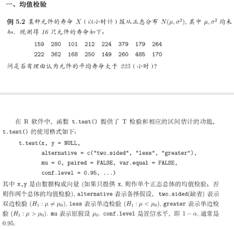
> t.test(X,alternative='greater',mu=225,conf.level = 0.95)#单边检验 One Sample t-test data: X
t = 0.66852, df = 15, p-value = 0.257
alternative hypothesis: true mean is greater than 225
95 percent confidence interval:
198.2321 Inf
sample estimates:
mean of x
241.5

> ###########################5.3这是一个经典的两样本比较问题
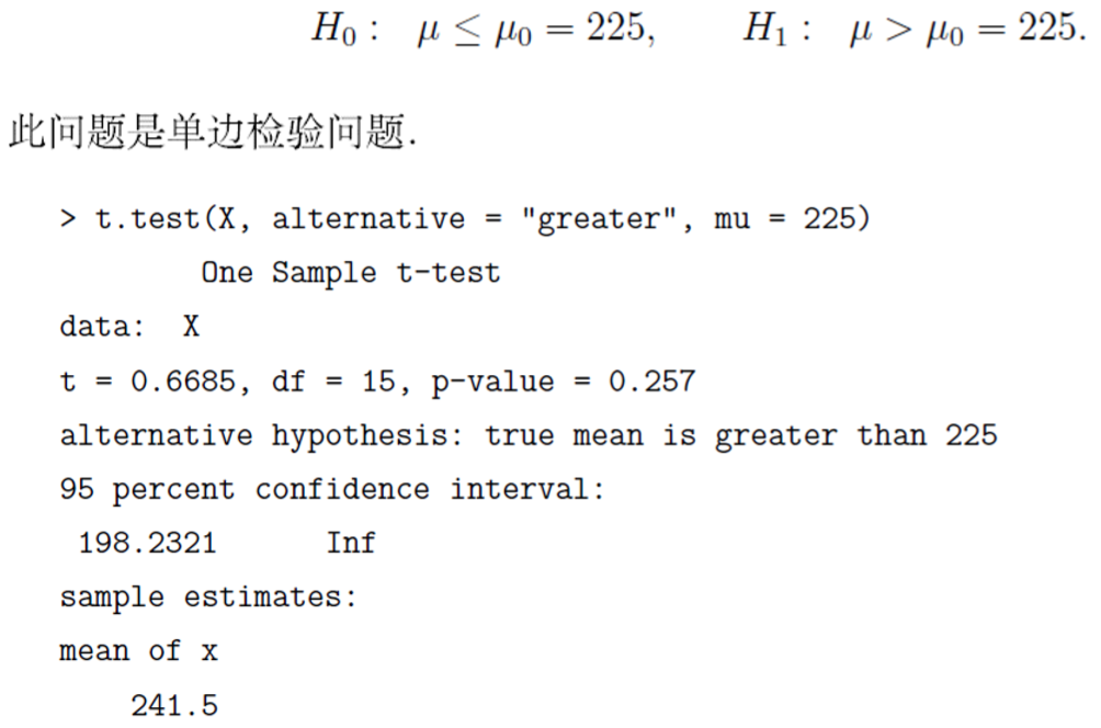
> X<-c(78.1, 72.4, 76.2, 74.3, 77.4, 78.4, 76.0, 75.5, 76.7, 77.3)
> Y<-c(79.1, 81.0, 77.3, 79.1, 80.0, 79.1, 79.1, 77.3, 80.2, 82.1)
> t.test(X,Y,var.equal=TRUE,alternative='less')#常把我们想要的结果作为备胎h1 Two Sample t-test data: X and Y
t = -4.2957, df = 18, p-value = 0.0002176
alternative hypothesis: true difference in means is less than 0
95 percent confidence interval:
-Inf -1.908255
sample estimates:
mean of x mean of y
76.23 79.43 > t.test(X,Y,var.equal=F,alternative='less')#两组样本方差不同 Welch Two Sample t-test data: X and Y
t = -4.2957, df = 17.319, p-value = 0.0002355
alternative hypothesis: true difference in means is less than 0
95 percent confidence interval:
-Inf -1.9055
sample estimates:
mean of x mean of y
76.23 79.43 > t.test(X,Y,var.equal=TRUE,alternative='less',paired=T)#两组样本数量相同 Paired t-test data: X and Y
t = -4.2018, df = 9, p-value = 0.00115
alternative hypothesis: true difference in means is less than 0
95 percent confidence interval:
-Inf -1.803943
sample estimates:
mean of the differences
-3.2
#实战我们将使用MASS包中的UScrime数据集。它包含了1960年美国47个州的刑 罚制度

#对犯罪率影响的信息。我们感兴趣的结果变量为Prob(监禁的概率)、U1(14~24岁年龄

#段城市男性失业率)和U2(35~39岁年龄段城市男性失业率)。类别型变量So(指示该州是

#否位 于南方的指示变量)将作为分组变量使用

#如果你在美国的南方犯罪,是否更有可能被判监禁?

install.packages("MASS")

library(MASS)

attach(UScrime)

t.test(Prob~So)#默认原假设为监禁概率相同

detach(UScrime)
方差检验
> ################################5.5方差检验

> X<-c(78.1, 72.4, 76.2, 74.3, 77.4, 78.4, 76.0, 75.5, 76.7, 77.3)

> Y<-c(79.1, 81.0, 77.3, 79.1, 80.0, 79.1, 79.1, 77.3, 80.2, 82.1)

> var.test(X,Y,alternative='two.side')

	F test to compare two variances

data:  X and Y

F = 1.4945, num df = 9, denom df = 9, p-value = 0.559

alternative hypothesis: true ratio of variances is not equal to 1

95 percent confidence interval:

 0.3712079 6.0167710

sample estimates:

ratio of variances

          1.494481

> ##############################5.6并非所有的样本总体都服从正态分布的假设!
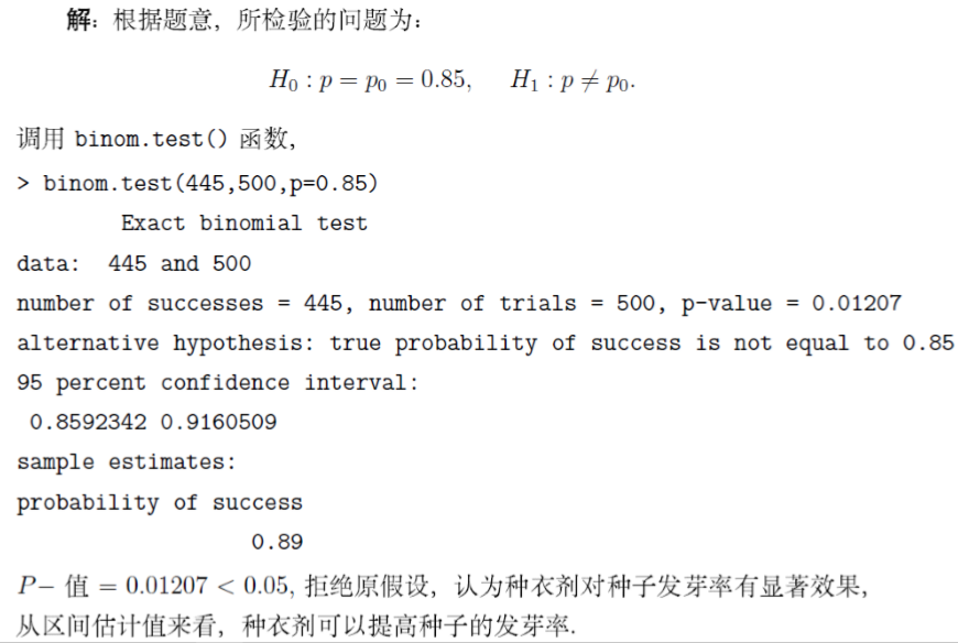
> binom.test(445,500,p=0.85) Exact binomial test data: 445 and 500
number of successes = 445, number of trials = 500, p-value = 0.01207
alternative hypothesis: true probability of success is not equal to 0.85
95 percent confidence interval:
0.8592342 0.9160509
sample estimates:
probability of success
0.89
#######5.7

binom.test(1,400,p=0.01,alternative='less')

##################5.8拟合优度检验

X=c(210,312,170,85,223)

chisq.test(X)

length(X)

######################5.12单个总体的检验

X<-c(420, 500, 920, 1380, 1510, 1650, 1760, 2100, 2300, 2350)

ks.test(X, "pexp", 1/1500)

?ks.test

########################两个样本分布的比较

X<-rnorm(100)

Y<-runif(100)

ks.test(X,Y)

t.test(X,Y)

wilcox.test(X,Y)

#################################################5.14列联表的独立性检验

x<-c(60, 3, 32, 11)

dim(x)<-c(2, 2)

x

chisq.test(x, correct = FALSE)#一个逻辑指示在计算2乘2表时的测试统计量时是否应用连续性校正
#实际例子

install.packages("vcd")#关节炎治疗数据

help(package='vcd')

library(vcd)

help("Arthritis")

head(Arthritis)#查看列表的前几项

mytable=xtabs(~Treatment+Improved,data=Arthritis);mytable#创建一个列联表。接受治疗和改善水平之间有关系

chisq.test(mytable)

fisher.test(mytable)

#改善水平和性别的关系

mytable=xtabs(~Improved+Sex,data=Arthritis);mytable

chisq.test(mytable)

fisher.test(mytable)

#多维度列联表的检验;原假设是两变量在第三个变量的每一层中都是条件独立的

mytable=xtabs(~Treatment+Improved+Sex,data=Arthritis)

mantelhaen.test(mytable)

#以上为独立性检验,如果变量独立,那么是否会相关呢?

library(vcd)#二维列联表相关性度量

mytable=xtabs(~Treatment+Improved,data=Arthritis);mytable

assocstats(mytable)

###############################5.22相关检验(相关性的度量)

x<-c(1,2,3,4,5,6); y<-c(6,5,4,3,2,1)

cor.test(x, y, method = "spearman")#还有person相关,kendall相关
实战
#实战

attach(state.x77)#基础包中的数据集,美国50个州在1977年的人口,收入,文盲率,预期寿命

#谋杀率,气温,土地面积等数据,我们想要判断预期寿命和谋杀率的关系

help(state.x77)

#install.packages("XQuartz");library(XQuartz);edit(state.x77);fix(state.x77)

head(state.x77)

states=state.x77[,1:6]#我们打算讨论除了气温和土地面积之外的所有变量的关系

cov(states)

cor(states)

pairs(state.x77)

cor.test(states[,4],states[,5])#预期寿命和谋杀率

detach(state.x77)

#cor.test 一次只能检验一对变量的相关性,而psych包中的corr.test()可以做的更多

library(psych)

corr.test(states,use='complete')#对所有变量做比较,prob 越小越显著
> states=state.x77[,1:6]#我们打算讨论除了气温和土地面积之外的所有变量的关系

> states

               Population Income Illiteracy Life Exp Murder HS Grad

Alabama              3615   3624        2.1    69.05   15.1    41.3

Alaska                365   6315        1.5    69.31   11.3    66.7

Arizona              2212   4530        1.8    70.55    7.8    58.1

Arkansas             2110   3378        1.9    70.66   10.1    39.9

California          21198   5114        1.1    71.71   10.3    62.6

Colorado             2541   4884        0.7    72.06    6.8    63.9

Connecticut          3100   5348        1.1    72.48    3.1    56.0

Delaware              579   4809        0.9    70.06    6.2    54.6

Florida              8277   4815        1.3    70.66   10.7    52.6

Georgia              4931   4091        2.0    68.54   13.9    40.6

Hawaii                868   4963        1.9    73.60    6.2    61.9

Idaho                 813   4119        0.6    71.87    5.3    59.5

Illinois            11197   5107        0.9    70.14   10.3    52.6

Indiana              5313   4458        0.7    70.88    7.1    52.9

Iowa                 2861   4628        0.5    72.56    2.3    59.0

Kansas               2280   4669        0.6    72.58    4.5    59.9

Kentucky             3387   3712        1.6    70.10   10.6    38.5

Louisiana            3806   3545        2.8    68.76   13.2    42.2

Maine                1058   3694        0.7    70.39    2.7    54.7

Maryland             4122   5299        0.9    70.22    8.5    52.3

Massachusetts        5814   4755        1.1    71.83    3.3    58.5

Michigan             9111   4751        0.9    70.63   11.1    52.8

Minnesota            3921   4675        0.6    72.96    2.3    57.6

Mississippi          2341   3098        2.4    68.09   12.5    41.0

Missouri             4767   4254        0.8    70.69    9.3    48.8

Montana               746   4347        0.6    70.56    5.0    59.2

Nebraska             1544   4508        0.6    72.60    2.9    59.3

Nevada                590   5149        0.5    69.03   11.5    65.2

New Hampshire         812   4281        0.7    71.23    3.3    57.6

New Jersey           7333   5237        1.1    70.93    5.2    52.5

New Mexico           1144   3601        2.2    70.32    9.7    55.2

New York            18076   4903        1.4    70.55   10.9    52.7

North Carolina       5441   3875        1.8    69.21   11.1    38.5

North Dakota          637   5087        0.8    72.78    1.4    50.3

Ohio                10735   4561        0.8    70.82    7.4    53.2

Oklahoma             2715   3983        1.1    71.42    6.4    51.6

Oregon               2284   4660        0.6    72.13    4.2    60.0

Pennsylvania        11860   4449        1.0    70.43    6.1    50.2

Rhode Island          931   4558        1.3    71.90    2.4    46.4

South Carolina       2816   3635        2.3    67.96   11.6    37.8

South Dakota          681   4167        0.5    72.08    1.7    53.3

Tennessee            4173   3821        1.7    70.11   11.0    41.8

Texas               12237   4188        2.2    70.90   12.2    47.4

Utah                 1203   4022        0.6    72.90    4.5    67.3

Vermont               472   3907        0.6    71.64    5.5    57.1

Virginia             4981   4701        1.4    70.08    9.5    47.8

Washington           3559   4864        0.6    71.72    4.3    63.5

West Virginia        1799   3617        1.4    69.48    6.7    41.6

Wisconsin            4589   4468        0.7    72.48    3.0    54.5

Wyoming               376   4566        0.6    70.29    6.9    62.9

> cov(states)

              Population      Income   Illiteracy     Life Exp      Murder      HS Grad

Population 19931683.7588 571229.7796  292.8679592 -407.8424612 5663.523714 -3551.509551

Income       571229.7796 377573.3061 -163.7020408  280.6631837 -521.894286  3076.768980

Illiteracy      292.8680   -163.7020    0.3715306   -0.4815122    1.581776    -3.235469

Life Exp       -407.8425    280.6632   -0.4815122    1.8020204   -3.869480     6.312685

Murder         5663.5237   -521.8943    1.5817755   -3.8694804   13.627465   -14.549616

HS Grad       -3551.5096   3076.7690   -3.2354694    6.3126849  -14.549616    65.237894

> cor(states)

            Population     Income Illiteracy    Life Exp     Murder     HS Grad

Population  1.00000000  0.2082276  0.1076224 -0.06805195  0.3436428 -0.09848975

Income      0.20822756  1.0000000 -0.4370752  0.34025534 -0.2300776  0.61993232

Illiteracy  0.10762237 -0.4370752  1.0000000 -0.58847793  0.7029752 -0.65718861

Life Exp   -0.06805195  0.3402553 -0.5884779  1.00000000 -0.7808458  0.58221620

Murder      0.34364275 -0.2300776  0.7029752 -0.78084575  1.0000000 -0.48797102

HS Grad    -0.09848975  0.6199323 -0.6571886  0.58221620 -0.4879710  1.00000000

> cor.test(states[,4],states[,5])#预期寿命和谋杀率

	Pearson's product-moment correlation

data:  states[, 4] and states[, 5]

t = -8.6596, df = 48, p-value = 2.26e-11

alternative hypothesis: true correlation is not equal to 0

95 percent confidence interval:

 -0.8700837 -0.6420442

sample estimates:

       cor

-0.7808458 #所以是负相关
> corr.test(states,use='complete')#对所有变量做比较,prob 越小越显著

Call:corr.test(x = states, use = "complete")

Correlation matrix

           Population Income Illiteracy Life Exp Murder HS Grad

Population       1.00   0.21       0.11    -0.07   0.34   -0.10

Income           0.21   1.00      -0.44     0.34  -0.23    0.62

Illiteracy       0.11  -0.44       1.00    -0.59   0.70   -0.66

Life Exp        -0.07   0.34      -0.59     1.00  -0.78    0.58

Murder           0.34  -0.23       0.70    -0.78   1.00   -0.49

HS Grad         -0.10   0.62      -0.66     0.58  -0.49    1.00

Sample Size

[1] 50

Probability values (Entries above the diagonal are adjusted for multiple tests.)

           Population Income Illiteracy Life Exp Murder HS Grad

Population       0.00   0.59       1.00      1.0   0.10       1

Income           0.15   0.00       0.01      0.1   0.54       0

Illiteracy       0.46   0.00       0.00      0.0   0.00       0

Life Exp         0.64   0.02       0.00      0.0   0.00       0

Murder           0.01   0.11       0.00      0.0   0.00       0

HS Grad          0.50   0.00       0.00      0.0   0.00       0

 To see confidence intervals of the correlations, print with the short=FALSE option
#以上大都是在讲两组比较,若是多组比较则需要方差分析的方法。这里仅介绍单因素方差分析

#多元方差分析参见《R语言实战》

#单因素方差分析中,你感兴趣的是比较分类因子定义的两个或多个组别中的因变量均值。以

#multcomp包中的cholesterol数据集为例(取自Westfall,Tobia,Rom,Hochberg,1999),

#50 个患者均接受降低胆固醇药物治疗(trt)五种疗法中的一种疗法。其中三种治疗条件使用药

#物相同,分别是20 mg一天一次(1time)、10 mg一天两次(2times)和5 mg一天四次(4times)。

#剩下的两种方式(drugD和drugE)代表候选药物。哪种药物疗法降低胆固醇(响应变量)最多呢?

install.packages('multcomp')

library(multcomp)

attach(cholesterol)

head(cholesterol)

table(trt)

fit=aov(response~trt);summary(fit)#方差分析只能看出它们之间的不同,不能说明具体细节

#绘图表示细节

boxplot(response~trt)

install.packages('gplots')

library(gplots)

plotmeans(response~trt,xlab='Treatment',ylab='Response',main='difference between 5 treatment')

detach(cholesterol)
所有代码:
####################5.2

X<-c(159, 280, 101, 212, 224, 379, 179, 264,

     222, 362, 168, 250, 149, 260, 485, 170)

t.test(X,alternative='greater',mu=225,conf.level = 0.95)#单边检验

###########################5.3这是一个经典的两样本比较问题

X<-c(78.1, 72.4, 76.2, 74.3, 77.4, 78.4, 76.0, 75.5, 76.7, 77.3)

Y<-c(79.1, 81.0, 77.3, 79.1, 80.0, 79.1, 79.1, 77.3, 80.2, 82.1)

t.test(X,Y,var.equal=TRUE,alternative='less')#常把我们想要的结果作为备胎h1

t.test(X,Y,var.equal=F,alternative='less')#两组样本方差不同

t.test(X,Y,var.equal=TRUE,alternative='less',paired=T)#两组样本数量相同

#实战我们将使用MASS包中的UScrime数据集。它包含了1960年美国47个州的刑 罚制度

#对犯罪率影响的信息。我们感兴趣的结果变量为Prob(监禁的概率)、U1(14~24岁年龄

#段城市男性失业率)和U2(35~39岁年龄段城市男性失业率)。类别型变量So(指示该州是

#否位 于南方的指示变量)将作为分组变量使用

#如果你在美国的南方犯罪,是否更有可能被判监禁?

install.packages("MASS")

library(MASS)

attach(UScrime)

t.test(Prob~So)#默认原假设为监禁概率相同

detach(UScrime)

################################5.5方差检验

X<-c(78.1, 72.4, 76.2, 74.3, 77.4, 78.4, 76.0, 75.5, 76.7, 77.3)

Y<-c(79.1, 81.0, 77.3, 79.1, 80.0, 79.1, 79.1, 77.3, 80.2, 82.1)

var.test(X,Y,alternative='two.side')

##############################5.6并非所有的样本总体都服从正态分布的假设!

binom.test(445,500,p=0.85)

#######5.7

binom.test(1,400,p=0.01,alternative='less')

##################5.8拟合优度检验

X=c(210,312,170,85,223)

chisq.test(X)

length(X)

######################5.12单个总体的检验

X<-c(420, 500, 920, 1380, 1510, 1650, 1760, 2100, 2300, 2350)

ks.test(X, "pexp", 1/1500)

?ks.test

########################两个样本分布的比较

X<-rnorm(100)

Y<-runif(100)

ks.test(X,Y)

t.test(X,Y)

wilcox.test(X,Y)

#################################################5.14列联表的独立性检验

x<-c(60, 3, 32, 11)

dim(x)<-c(2, 2)

x

chisq.test(x, correct = FALSE)#一个逻辑指示在计算2乘2表时的测试统计量时是否应用连续性校正

#实际例子

install.packages("vcd")#关节炎治疗数据

help(package='vcd')

library(vcd)

help("Arthritis")

head(Arthritis)#查看列表的前几项

mytable=xtabs(~Treatment+Improved,data=Arthritis);mytable#创建一个列联表。接受治疗和改善水平之间有关系

chisq.test(mytable)

fisher.test(mytable)

#改善水平和性别的关系

mytable=xtabs(~Improved+Sex,data=Arthritis);mytable

chisq.test(mytable)

fisher.test(mytable)

#多维度列联表的检验;原假设是两变量在第三个变量的每一层中都是条件独立的

mytable=xtabs(~Treatment+Improved+Sex,data=Arthritis)

mantelhaen.test(mytable)

#以上为独立性检验,如果变量独立,那么是否会相关呢?

library(vcd)#二维列联表相关性度量

mytable=xtabs(~Treatment+Improved,data=Arthritis);mytable

assocstats(mytable)

###############################5.22相关检验(相关性的度量)

x<-c(1,2,3,4,5,6); y<-c(6,5,4,3,2,1)

cor.test(x, y, method = "spearman")#还有person相关,kendall相关

#实战

attach(state.x77)#基础包中的数据集,美国50个州在1977年的人口,收入,文盲率,预期寿命

#谋杀率,气温,土地面积等数据,我们想要判断预期寿命和谋杀率的关系

help(state.x77)

#install.packages("XQuartz");library(XQuartz);edit(state.x77);fix(state.x77)

head(state.x77)

states=state.x77[,1:6]#我们打算讨论除了气温和土地面积之外的所有变量的关系

cov(states)

cor(states)

pairs(state.x77)

cor.test(states[,4],states[,5])#预期寿命和谋杀率

detach(state.x77)

#cor.test 一次只能检验一对变量的相关性,而psych包中的corr.test()可以做的更多

library(psych)

corr.test(states,use='complete')#对所有变量做比较,prob 越小越显著

#以上大都是在讲两组比较,若是多组比较则需要方差分析的方法。这里仅介绍单因素方差分析

#多元方差分析参见《R语言实战》

#单因素方差分析中,你感兴趣的是比较分类因子定义的两个或多个组别中的因变量均值。以

#multcomp包中的cholesterol数据集为例(取自Westfall,Tobia,Rom,Hochberg,1999),

#50 个患者均接受降低胆固醇药物治疗(trt)五种疗法中的一种疗法。其中三种治疗条件使用药

#物相同,分别是20 mg一天一次(1time)、10 mg一天两次(2times)和5 mg一天四次(4times)。

#剩下的两种方式(drugD和drugE)代表候选药物。哪种药物疗法降低胆固醇(响应变量)最多呢?

install.packages('multcomp')

library(multcomp)

attach(cholesterol)

head(cholesterol)

table(trt)

fit=aov(response~trt);summary(fit)#方差分析只能看出它们之间的不同,不能说明具体细节

#绘图表示细节

boxplot(response~trt)

install.packages('gplots')

library(gplots)

plotmeans(response~trt,xlab='Treatment',ylab='Response',main='difference between 5 treatment')

detach(cholesterol)
R语言与概率统计(二) 假设检验的更多相关文章
- R语言结合概率统计的体系分析---数字特征
现在有一个人,如何对这个人怎么识别这个人?那么就对其存在的特征进行提取,比如,提取其身高,其相貌,其年龄,分析这些特征,从而确定了,这个人就是这个人,我们绝不会认错. 同理,对数据进行分析,也是提取出 ...
- R语言与概率统计(一) 描述性统计分析
#查看已安装的包,查看已载入的包,查看包的介绍 ########例题3.1 #向量的输入方法 w<-c(75.0, 64.0, 47.4, 66.9, 62.2, 62.2, 58.7, 6 ...
- R语言与概率统计(六) 主成分分析 因子分析
超高维度分析,N*P的矩阵,N为样本个数,P为指标,N<<P PCA:抓住对y对重要的影响因素 主要有三种:PCA,因子分析,回归方程+惩罚函数(如LASSO) 为了降维,用更少的变量解决 ...
- R语言与概率统计(五) 聚类分析
#########################################0808聚类分析 X<-data.frame( x1=c(2959.19, 2459.77, 1495.63, ...
- R语言与概率统计(四) 判别分析(分类)
Fisher就是找一个线L使得组内方差小,组间距离大.即找一个直线使得d最大. ####################################1.判别分析,线性判别:2.分层抽样 #inst ...
- R语言与概率统计(三) 多元统计分析(下)广义线性回归
广义线性回归 > life<-data.frame( + X1=c(2.5, 173, 119, 10, 502, 4, 14.4, 2, 40, 6.6, + 21.4, 2.8, 2. ...
- R语言与概率统计(三) 多元统计分析(中)
模型修正 #但是,回归分析通常很难一步到位,需要不断修正模型 ###############################6.9通过牙膏销量模型学习模型修正 toothpaste<-data. ...
- R语言与概率统计(三) 多元统计分析(上)
> #############6.2一元线性回归分析 > x<-c(0.10,0.11,0.12,0.13,0.14,0.15,0.16,0.17,0.18,0.20,0.21,0. ...
- R语言基础入门之二:数据导入和描述统计
by 写长城的诗 • October 30, 2011 • Comments Off This post was kindly contributed by 数据科学与R语言 - go there t ...
随机推荐
- bug是前端还是后端
分析bug是前端还是后端的 如何分析一个bug是前端还是后端的? 平常提bug的时候,前端开发和后端开发总是扯皮,不承认是对方的bug这种情况很容易判断,先抓包看请求报文,对着接口文档,看请求报文 ...
- HAL UART DMA 数据收发
UART使用DMA进行数据收发,实现功能,串口2发送指令到上位机,上位机返回数据给串口2,串口2收到数据后由串口1进行转发,该功能为实验功能 1.UART与DMA通道进行绑定 void HAL_UAR ...
- wkhtmltopdf 自定义字体未生效或中文乱码
使用wkhtmltopdf控件将网页保存成pdf的过程中出现网页中有些字体,在PDF中未生效.通过网上查询结果有一种处理方式: 在网页头部的style标签中,手工指定宋体字体的本地存放位置,wkhtm ...
- 微信小程序开发框架 Wepy 的使用
一.github地址:https://github.com/Tencent/wepy 按照 README.md 的步骤进行操作: 1.在“介绍”中获得 wepy 的开发资源汇总:https://git ...
- Redis之哨兵机制(五)
什么是哨兵机制 Redis的哨兵(sentinel) 系统用于管理多个 Redis 服务器,该系统执行以下三个任务: · 监控(Monitoring): 哨兵(sentinel) 会不断 ...
- centos 解决 mysql command not found
执行命令: mysql -V 报错内容: -bash: mysql: command not found 报错原因:系统默认会查找/usr/bin下的命令,如果这个命令不在这个目录下,当然会找不到命令 ...
- python之select与selector
select/poll/epoll的区别 I/O多路复用的本质就是用select/poll/epoll,去监听多个socket对象. 参考:Linux IO模式及 select.poll.epoll详 ...
- VSCODE常用插件使用记录
常用必备: 1.vscode-icon 让 vscode 资源树目录加上图标,必备良品! 2.Path Intellisense 自动路劲补全,默认不带这个功能的 3.beautify Beautif ...
- 洛谷P1363 幻想迷宫【dfs】
题目:https://www.luogu.org/problemnew/show/P1363 题意: 有一个地图,起点是S,障碍物用#表示.可以将这个地图不断的在四周重复,问从起点开始是否可以走到无限 ...
- error MSB6006: “cmd.exe”已退出,代码为 3。
error MSB6006: “cmd.exe”已退出,代码为 3. 这两天调程序遇到一个奇怪的问题. C:\Program Files (x86)\MSBuild\Microsoft.Cpp\v4. ...