Importing data in R 1

目录

• Importing data in R 学习笔记1
  • flat files:CSV
  • txt文件
  • packages：readr
    • read_csv()
  • read_tsv
    • read_delim()
  • data.table()
    • fread
  • readxl
    • excel_sheets()
    • read_excel()
  • gdata
    • read.xls()
    • getSheets()
  • XLConnect
    • loadWorkbook()
    • readWorksheet（）
    • createSheet()
    • writeWorksheet()
    • saveWorkbook
    • renameSheet()
    • removeSheet()

Importing data in R 学习笔记1

flat files:CSV

# Import swimming_pools.csv correctly: pools
pools<-read.csv("swimming_pools.csv",stringsAsFactors=FALSE)

txt文件

read.delim("name.txt",header=TRUE)

转化为table
# Path to the hotdogs.txt file: path
> path <- file.path("data", "hotdogs.txt")
>
> # Import the hotdogs.txt file: hotdogs
> hotdogs <- read.table(path,
                        sep = "\t",
                        col.names = c("type", "calories", "sodium"))
>
> # Call head() on hotdogs
> head(hotdogs)
  type calories sodium
1 Beef      186    495
2 Beef      181    477
3 Beef      176    425
4 Beef      149    322
5 Beef      184    482
6 Beef      190    587

tibble:简单数据框

read_对比read.

前者产生一个简单的数据框，并且会展示每一列的数据类型

packages：readr

read_csv()

读入csv格式

read_csv and read_tsv are special cases of the general read_delim. They're useful for reading the most common types of flat file data, comma separated values and tab separated values, respectively. read_csv2 uses ; for separators, instead of ,. This is common in European countries which use , as the decimal separator

read_tsv

读入txt格式

> # readr is already loaded
>
> # Column names
> properties <- c("area", "temp", "size", "storage", "method",
                  "texture", "flavor", "moistness")
>
> # Import potatoes.txt: potatoes
读入数据并指定行名
> potatoes<-read_tsv("potatoes.txt",col_names=properties)
Parsed with column specification:
cols(
  area = col_integer(),
  temp = col_integer(),
  size = col_integer(),
  storage = col_integer(),
  method = col_integer(),
  texture = col_double(),
  flavor = col_double(),
  moistness = col_double()
)
> col_names=properties
>
> # Call head() on potatoes
> head(potatoes)
# A tibble: 6 x 8
   area  temp  size storage method texture flavor moistness
  <int> <int> <int>   <int>  <int>   <dbl>  <dbl>     <dbl>
1     1     1     1       1      1     2.9    3.2       3
2     1     1     1       1      2     2.3    2.5       2.6
3     1     1     1       1      3     2.5    2.8       2.8
4     1     1     1       1      4     2.1    2.9       2.4
5     1     1     1       1      5     1.9    2.8       2.2
6     1     1     1       2      1     1.8    3         1.7

read_delim()

# Column names
> properties <- c("area", "temp", "size", "storage", "method",
                  "texture", "flavor", "moistness")
>
> # Import potatoes.txt using read_delim(): potatoes
> potatoes <- read_delim("potatoes.txt", delim = "\t", col_names = properties)
Parsed with column specification:
cols(
  area = col_integer(),
  temp = col_integer(),
  size = col_integer(),
  storage = col_integer(),
  method = col_integer(),
  texture = col_double(),
  flavor = col_double(),
  moistness = col_double()
)
>
> # Print out potatoes
> potatoes
# A tibble: 160 x 8
    area  temp  size storage method texture flavor moistness
   <int> <int> <int>   <int>  <int>   <dbl>  <dbl>     <dbl>
 1     1     1     1       1      1     2.9    3.2       3
 2     1     1     1       1      2     2.3    2.5       2.6
 3     1     1     1       1      3     2.5    2.8       2.8
 4     1     1     1       1      4     2.1    2.9       2.4
 5     1     1     1       1      5     1.9    2.8       2.2
 6     1     1     1       2      1     1.8    3         1.7
 7     1     1     1       2      2     2.6    3.1       2.4
 8     1     1     1       2      3     3      3         2.9
 9     1     1     1       2      4     2.2    3.2       2.5
10     1     1     1       2      5     2      2.8       1.9
# ... with 150 more rows

data.table()

fread

make up some column names itself

more convenience

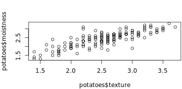
 # Import columns 6 and 8 of potatoes.csv: potatoes
> potatoes<-fread("potatoes.csv",select=c(6,8))
>
> # Plot texture (x) and moistness (y) of potatoes
> plot(potatoes$texture,potatoes$moistness)

readxl

excel_sheets()

library(readxl)
# Print the names of all worksheets
excel_sheets("urbanpop.xlsx")

# Read all Excel sheets with lapply(): pop_list
pop_list<- lapply(excel_sheets("urbanpop.xlsx"),
                      read_excel,
                      path = "urbanpop.xlsx")

# Display the structure of pop_list
str(pop_list)

read_excel()

# Import the second sheet of urbanpop.xlsx, skipping the first 21 rows: urbanpop_sel
urbanpop_sel <- read_excel("urbanpop.xlsx", sheet = 2, col_names = FALSE, skip = 21)

# Print out the first observation from urbanpop_sel
urbanpop_sel[1,]

gdata

read.xls()

读入xls格式的数据

# Column names for urban_pop
> columns <- c("country", paste0("year_", 1967:1974))
>
> # Finish the read.xls call
> urban_pop <- read.xls("urbanpop.xls", sheet = 2,
                        skip = 50, header = FALSE, stringsAsFactors = FALSE,
                        col.names = columns)
>
> # Print first 10 observation of urban_pop
> head(urban_pop,n=10)
              country   year_1967   year_1968   year_1969   year_1970
1              Cyprus   231929.74   237831.38   243983.34   250164.52
2      Czech Republic  6204409.91  6266304.50  6326368.97  6348794.89
3             Denmark  3777552.62  3826785.08  3874313.99  3930042.97
4            Djibouti    77788.04    84694.35    92045.77    99845.22
5            Dominica    27550.36    29527.32    31475.62    33328.25
6  Dominican Republic  1535485.43  1625455.76  1718315.40  1814060.00
7             Ecuador  2059355.12  2151395.14  2246890.79  2345864.41
8               Egypt 13798171.00 14248342.19 14703858.22 15162858.52
9         El Salvador  1345528.98  1387218.33  1429378.98  1472181.26
10  Equatorial Guinea    75364.50    77295.03    78445.74    78411.07
     year_1971   year_1972   year_1973   year_1974
1    261213.21   272407.99   283774.90   295379.83
2   6437055.17  6572632.32  6718465.53  6873458.18
3   3981360.12  4028247.92  4076867.28  4120201.43
4    107799.69   116098.23   125391.58   136606.25
5     34761.52    36049.99    37260.05    38501.47
6   1915590.38  2020157.01  2127714.45  2238203.87
7   2453817.78  2565644.81  2681525.25  2801692.62
8  15603661.36 16047814.69 16498633.27 16960827.93
9   1527985.34  1584758.18  1642098.95  1699470.87
10    77055.29    74596.06    71438.96    68179.26

getSheets()

查看一个excel文件有多少的sheet，输出每个sheet的名字

XLConnect

loadWorkbook()

主要是加载excel文件

When working with XLConnect, the first step will be to load a workbook in your R session with loadWorkbook(); this function will build a "bridge" between your Excel file and your R session.

library("XLConnect")
>
> # Build connection to urbanpop.xlsx: my_book
> my_book<-loadWorkbook("urbanpop.xlsx")
>
> # Print out the class of my_book
> class(my_book)
[1] "workbook"
attr(,"package")
[1] "XLConnect"

readWorksheet（）

读取excel文件

所以顺序肯定是先加载再读取啊。

# Import columns 3, 4, and 5 from second sheet in my_book: urbanpop_sel
urbanpop_sel <- readWorksheet(my_book, sheet = 2,startCol=3,endCol=5)

# Import first column from second sheet in my_book: countries
countries<-readWorksheet(my_book, sheet = 2,startCol=1,endCol=1)

# cbind() urbanpop_sel and countries together: selection
selection<-cbind(countries,urbanpop_sel)

createSheet()

在已经有的excel中创建一个sheet，创建一个空的sheet

# Build connection to urbanpop.xlsx
> my_book <- loadWorkbook("urbanpop.xlsx")
>
> # Add a worksheet to my_book, named "data_summary"
> createSheet(my_book,"data_summary")
>
> # Use getSheets() on my_book
> getSheets(my_book)
[1] "1960-1966"    "1967-1974"    "1975-2011"    "data_summary"

writeWorksheet()

Writes data to worksheets of a '>workbook.

saveWorkbook

保存工作表，就是存到磁盘上

# Build connection to urbanpop.xlsx
my_book <- loadWorkbook("urbanpop.xlsx")

# Add a worksheet to my_book, named "data_summary"
createSheet(my_book, "data_summary")

# Create data frame: summ
sheets <- getSheets(my_book)[1:3]
dims <- sapply(sheets, function(x) dim(readWorksheet(my_book, sheet = x)), USE.NAMES = FALSE)
summ <- data.frame(sheets = sheets,
                   nrows = dims[1, ],
                   ncols = dims[2, ])

# Add data in summ to "data_summary" sheet
writeWorksheet(my_book,summ,"data_summary")

# Save workbook as summary.xlsx
 saveWorkbook(my_book,"summary.xlsx")

renameSheet()

给sheet表重命名

# Rename "data_summary" sheet to "summary"
renameSheet(my_book, "data_summary", "summary")

# Print out sheets of my_book
getSheets(my_book)

# Save workbook to "renamed.xlsx"
saveWorkbook(my_book, file = "renamed.xlsx")

我发现我自己真的很容易丢参数哦，然后死活调不出来。。。===。。。苦恼的人儿

removeSheet()

删除指定sheet

library(XLConnect)
# Build connection to renamed.xlsx: my_book
my_book<-loadWorkbook("renamed.xlsx")

# Remove the fourth sheet
removeSheet(my_book,sheet="summary")

# Save workbook to "clean.xlsx"
saveWorkbook(my_book,"clean.xlsx")