ES进阶--04

第30节彻底掌握IK中文分词_上机动手实战IK中文分词器的安装和使用

之前大家会发现，我们全部是用英文在玩儿。。。好玩儿不好玩儿。。。不好玩儿

中国人，其实我们用来进行搜索的，绝大多数，都是中文应用，很少做英文的
standard：没有办法对中文进行合理分词的，只是将每个中文字符一个一个的切割开来，比如说中国人 --> 中 国 人

英语的也要学：所以说，我们利用核心知识篇的相关的知识，来把es这种英文原生的搜索引擎，先学一下; 因为有些知识点，可能用英文讲更靠谱，因为比如说analyzed，palyed，students --> stemmer，analyze，play，student。有些知识点，仅仅适用于英文，不太适用于中文

从这一讲开始，大家就会觉得很爽，因为全部都是我们熟悉的中文了，没有英文了，高阶知识点，搜索，聚合，全部是中文了

在搜索引擎领域，比较成熟和流行的，就是ik分词器

中国人很喜欢吃油条

standard：中 国 人 很 喜 欢 吃 油 条
ik：中国人 很 喜欢 吃 油条

1、在elasticsearch中安装ik中文分词器

（1）git clone https://github.com/medcl/elasticsearch-analysis-ik
（2）git checkout tags/v5.2.0
（3）mvn package
（4）将target/releases/elasticsearch-analysis-ik-5.2.0.zip拷贝到es/plugins/ik目录下
（5）在es/plugins/ik下对elasticsearch-analysis-ik-5.2.0.zip进行解压缩
（6）重启es

2、ik分词器基础知识

两种analyzer，你根据自己的需要自己选吧，但是一般是选用ik_max_word

ik_max_word: 会将文本做最细粒度的拆分，比如会将“中华人民共和国国歌”拆分为“中华人民共和国,中华人民,中华,华人,人民共和国,人民,人,民,共和国,共和,和,国国,国歌”，会穷尽各种可能的组合；

ik_smart: 会做最粗粒度的拆分，比如会将“中华人民共和国国歌”拆分为“中华人民共和国,国歌”。

共和国 --> 中华人民共和国和国歌，搜到吗？？？？

3、ik分词器的使用

PUT /my_index
{
"mappings": {
"my_type": {
"properties": {
"text": {
"type": "text",
"analyzer": "ik_max_word"
}
}
}
}
}

POST /my_index/my_type/_bulk
{ "index": { "_id": "1"} }
{ "text": "男子偷上万元发红包求交女友 被抓获时仍然单身" }
{ "index": { "_id": "2"} }
{ "text": "16岁少女为结婚“变”22岁 7年后想离婚被法院拒绝" }
{ "index": { "_id": "3"} }
{ "text": "深圳女孩骑车逆行撞奔驰 遭索赔被吓哭(图)" }
{ "index": { "_id": "4"} }
{ "text": "女人对护肤品比对男票好？网友神怼" }
{ "index": { "_id": "5"} }
{ "text": "为什么国内的街道招牌用的都是红黄配？" }

GET /my_index/_analyze
{
"text": "男子偷上万元发红包求交女友 被抓获时仍然单身",
"analyzer": "ik_max_word"
}

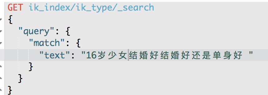
GET /my_index/my_type/_search
{
"query": {
"match": {
"text": "16岁少女结婚好还是单身好？"
}
}
}

第31节彻底掌握IK中文分词_IK分词器配置文件讲解以及自定义词库实战

1、ik配置文件

ik配置文件地址：es/plugins/ik/config目录

IKAnalyzer.cfg.xml：用来配置自定义词库
main.dic：ik原生内置的中文词库，总共有27万多条，只要是这些单词，都会被分在一起
quantifier.dic：放了一些单位相关的词
suffix.dic：放了一些后缀
surname.dic：中国的姓氏
stopword.dic：英文停用词

ik原生最重要的两个配置文件

main.dic：包含了原生的中文词语，会按照这个里面的词语去分词
stopword.dic：包含了英文的停用词

停用词，stopword

a the and at but

一般，像停用词，会在分词的时候，直接被干掉，不会建立在倒排索引中

2、自定义词库

（1）自己建立词库：每年都会涌现一些特殊的流行词，网红，蓝瘦香菇，喊麦，鬼畜，一般不会在ik的原生词典里

自己补充自己的最新的词语，到ik的词库里面去

IKAnalyzer.cfg.xml：ext_dict，custom/mydict.dic

补充自己的词语，然后需要重启es，才能生效

（2）自己建立停用词库：比如了，的，啥，么，我们可能并不想去建立索引，让人家搜索

custom/ext_stopword.dic，已经有了常用的中文停用词，可以补充自己的停用词，然后重启es

第32节彻底掌握IK中文分词_修改IK分词器源码来基于mysql热更新词库

热更新

每次都是在es的扩展词典中，手动添加新词语，很坑
（1）每次添加完，都要重启es才能生效，非常麻烦
（2）es是分布式的，可能有数百个节点，你不能每次都一个一个节点上面去修改

es不停机，直接我们在外部某个地方添加新的词语，es中立即热加载到这些新词语

热更新的方案

（1）修改ik分词器源码，然后手动支持从mysql中每隔一定时间，自动加载新的词库
（2）基于ik分词器原生支持的热更新方案，部署一个web服务器，提供一个http接口，通过modified和tag两个http响应头，来提供词语的热更新

用第一种方案，第二种，ik git社区官方都不建议采用，觉得不太稳定

1、下载源码

https://github.com/medcl/elasticsearch-analysis-ik/tree/v5.2.0

ik分词器，是个标准的java maven工程，直接导入eclipse就可以看到源码

2、修改源码

Dictionary类，169行：Dictionary单例类的初始化方法，在这里需要创建一个我们自定义的线程，并且启动它
HotDictReloadThread类：就是死循环，不断调用Dictionary.getSingleton().reLoadMainDict()，去重新加载词典
Dictionary类，389行：this.loadMySQLExtDict();
Dictionary类，683行：this.loadMySQLStopwordDict();

3、mvn package打包代码

target\releases\elasticsearch-analysis-ik-5.2.0.zip

4、解压缩ik压缩包

将mysql驱动jar，放入ik的目录下

5、修改jdbc相关配置

6、重启es

观察日志，日志中就会显示我们打印的那些东西，比如加载了什么配置，加载了什么词语，什么停用词

7、在mysql中添加词库与停用词

8、分词实验，验证热更新生效

第33节深入聚合数据分析_bucket与metric两个核心概念的讲解

课程大纲

1、文本编辑器介绍

（1）windows操作系统，原生的txt文本编辑器，一些json格式，不太方便去调整
（2）notepad++，功能不是太丰富
（3）sublime，整个功能也比较丰富，比较好，自己可以上网去下载，官网，免费的

2、两个核心概念：bucket和metric

bucket：一个数据分组   bucket 桶

city name

北京 小李
北京 小王
上海 小张
上海 小丽
上海 小陈

基于city划分buckets

划分出来两个bucket，一个是北京bucket，一个是上海bucket

北京bucket：包含了2个人，小李，小王
上海bucket：包含了3个人，小张，小丽，小陈

按照某个字段进行bucket划分，那个字段的值相同的那些数据，就会被划分到一个bucket中

有一些mysql的sql知识的话，聚合，首先第一步就是分组，对每个组内的数据进行聚合分析，分组，就是我们的bucket

metric：对一个数据分组执行的统计

当我们有了一堆bucket之后，就可以对每个bucket中的数据进行聚合分词了，比如说计算一个bucket内所有数据的数量，或者计算一个bucket内所有数据的平均值，最大值，最小值

metric，就是对一个bucket执行的某种聚合分析的操作，比如说求平均值，求最大值，求最小值

select count(*)
from access_log
group by user_id

bucket：group by user_id --> 那些user_id相同的数据，就会被划分到一个bucket中
metric：count(*)，对每个user_id bucket中所有的数据，计算一个数量

第34节深入聚合数据分析_家电卖场案例以及统计哪种颜色电视销量最高

课程大纲

1、家电卖场案例背景

以一个家电卖场中的电视销售数据为背景，来对各种品牌，各种颜色的电视的销量和销售额，进行各种各样角度的分析

PUT /tvs
{
"mappings": {
"sales": {
"properties": {
"price": {
"type": "long"
},
"color": {
"type": "keyword"
},
"brand": {
"type": "keyword"
},
"sold_date": {
"type": "date"
}
}
}
}
}

POST /tvs/sales/_bulk
{ "index": {}}
{ "price" : 1000, "color" : "红色", "brand" : "长虹", "sold_date" : "2016-10-28" }
{ "index": {}}
{ "price" : 2000, "color" : "红色", "brand" : "长虹", "sold_date" : "2016-11-05" }
{ "index": {}}
{ "price" : 3000, "color" : "绿色", "brand" : "小米", "sold_date" : "2016-05-18" }
{ "index": {}}
{ "price" : 1500, "color" : "蓝色", "brand" : "TCL", "sold_date" : "2016-07-02" }
{ "index": {}}
{ "price" : 1200, "color" : "绿色", "brand" : "TCL", "sold_date" : "2016-08-19" }
{ "index": {}}
{ "price" : 2000, "color" : "红色", "brand" : "长虹", "sold_date" : "2016-11-05" }
{ "index": {}}
{ "price" : 8000, "color" : "红色", "brand" : "三星", "sold_date" : "2017-01-01" }
{ "index": {}}
{ "price" : 2500, "color" : "蓝色", "brand" : "小米", "sold_date" : "2017-02-12" }

2、统计哪种颜色的电视销量最高

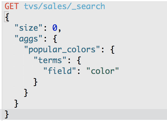
GET /tvs/sales/_search
{
"size" : 0,
"aggs" : {
"popular_colors" : {
"terms" : {
"field" : "color"
}
}
}
}

size：只获取聚合结果，而不要执行聚合的原始数据
aggs：固定语法，要对一份数据执行分组聚合操作
popular_colors：就是对每个aggs，都要起一个名字，这个名字是随机的，你随便取什么都ok
terms：根据字段的值进行分组
field：根据指定的字段的值进行分组

{
"took": 61,
"timed_out": false,
"_shards": {
"total": 5,
"successful": 5,
"failed": 0
},
"hits": {
"total": 8,
"max_score": 0,
"hits": []
},
"aggregations": {
"popular_color": {
"doc_count_error_upper_bound": 0,
"sum_other_doc_count": 0,
"buckets": [
{
"key": "红色",
"doc_count": 4
},
{
"key": "绿色",
"doc_count": 2
},
{
"key": "蓝色",
"doc_count": 2
}
]
}
}
}

hits.hits：我们指定了size是0，所以hits.hits就是空的，否则会把执行聚合的那些原始数据给你返回回来
aggregations：聚合结果
popular_color：我们指定的某个聚合的名称
buckets：根据我们指定的field划分出的buckets
key：每个bucket对应的那个值
doc_count：这个bucket分组内，有多少个数据
数量，其实就是这种颜色的销量

每种颜色对应的bucket中的数据的
默认的排序规则：按照doc_count降序排序

第35节深入聚合数据分析_实战bucket+metric：统计每种颜色电视平均价格

课程大纲

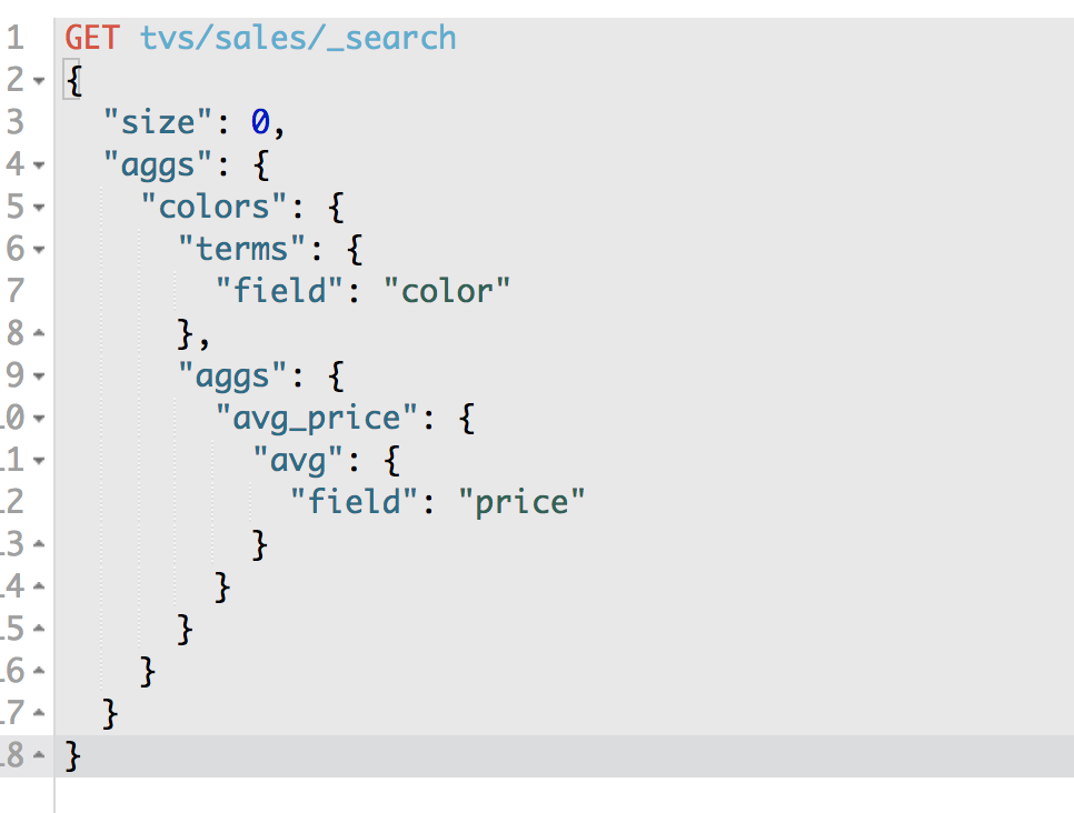
GET /tvs/sales/_search
{
"size" : 0,
"aggs": {
"colors": {
"terms": {
"field": "color"
},
"aggs": {
"avg_price": {
"avg": {
"field": "price"
}
}
}
}
}
}

按照color去分bucket，可以拿到每个color bucket中的数量，这个仅仅只是一个bucket操作，doc_count其实只是es的bucket操作默认执行的一个内置metric

这一讲，就是除了bucket操作，分组，还要对每个bucket执行一个metric聚合统计操作

在一个aggs执行的bucket操作（terms），平级的json结构下，再加一个aggs，这个第二个aggs内部，同样取个名字，执行一个metric操作，avg，对之前的每个bucket中的数据的指定的field，price field，求一个平均值

"aggs": {
"avg_price": {
"avg": {
"field": "price"
}
}
}

就是一个metric，就是一个对一个bucket分组操作之后，对每个bucket都要执行的一个metric

第一个metric，avg，求指定字段的平均值

{
"took": 28,
"timed_out": false,
"_shards": {
"total": 5,
"successful": 5,
"failed": 0
},
"hits": {
"total": 8,
"max_score": 0,
"hits": []
},
"aggregations": {
"group_by_color": {
"doc_count_error_upper_bound": 0,
"sum_other_doc_count": 0,
"buckets": [
{
"key": "红色",
"doc_count": 4,
"avg_price": {
"value": 3250
}
},
{
"key": "绿色",
"doc_count": 2,
"avg_price": {
"value": 2100
}
},
{
"key": "蓝色",
"doc_count": 2,
"avg_price": {
"value": 2000
}
}
]
}
}
}

buckets，除了key和doc_count
avg_price：我们自己取的metric aggs的名字
value：我们的metric计算的结果，每个bucket中的数据的price字段求平均值后的结果

select avg(price)
from tvs.sales
group by color

第36节深入聚合数据分析_bucket嵌套实现颜色+品牌的多层下钻分析

课程大纲

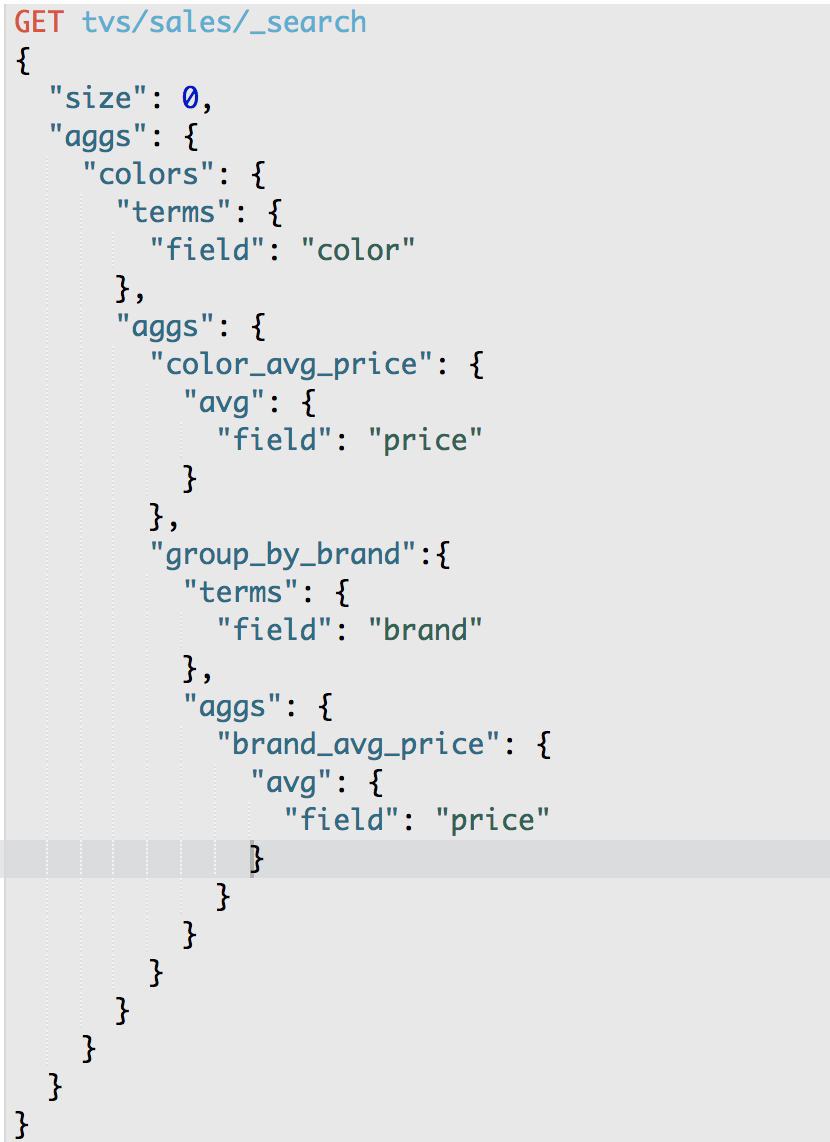
从颜色到品牌进行下钻分析，每种颜色的平均价格，以及找到每种颜色每个品牌的平均价格

我们可以进行多层次的下钻

比如说，现在红色的电视有4台，同时这4台电视中，有3台是属于长虹的，1台是属于小米的

红色电视中的3台长虹的平均价格是多少？
红色电视中的1台小米的平均价格是多少？

下钻的意思是，已经分了一个组了，比如说颜色的分组，然后还要继续对这个分组内的数据，再分组，比如一个颜色内，还可以分成多个不同的品牌的组，最后对每个最小粒度的分组执行聚合分析操作，这就叫做下钻分析

es，下钻分析，就要对bucket进行多层嵌套，多次分组

按照多个维度（颜色+品牌）多层下钻分析，而且学会了每个下钻维度（颜色，颜色+品牌），都可以对每个维度分别执行一次metric聚合操作

GET /tvs/sales/_search
{
"size": 0,
"aggs": {
"group_by_color": {
"terms": {
"field": "color"
},
"aggs": {
"color_avg_price": {
"avg": {
"field": "price"
}
},
"group_by_brand": {
"terms": {
"field": "brand"
},
"aggs": {
"brand_avg_price": {
"avg": {
"field": "price"
}
}
}
}
}
}
}
}

{
"took": 8,
"timed_out": false,
"_shards": {
"total": 5,
"successful": 5,
"failed": 0
},
"hits": {
"total": 8,
"max_score": 0,
"hits": []
},
"aggregations": {
"group_by_color": {
"doc_count_error_upper_bound": 0,
"sum_other_doc_count": 0,
"buckets": [
{
"key": "红色",
"doc_count": 4,
"color_avg_price": {
"value": 3250
},
"group_by_brand": {
"doc_count_error_upper_bound": 0,
"sum_other_doc_count": 0,
"buckets": [
{
"key": "长虹",
"doc_count": 3,
"brand_avg_price": {
"value": 1666.6666666666667
}
},
{
"key": "三星",
"doc_count": 1,
"brand_avg_price": {
"value": 8000
}
}
]
}
},
{
"key": "绿色",
"doc_count": 2,
"color_avg_price": {
"value": 2100
},
"group_by_brand": {
"doc_count_error_upper_bound": 0,
"sum_other_doc_count": 0,
"buckets": [
{
"key": "TCL",
"doc_count": 1,
"brand_avg_price": {
"value": 1200
}
},
{
"key": "小米",
"doc_count": 1,
"brand_avg_price": {
"value": 3000
}
}
]
}
},
{
"key": "蓝色",
"doc_count": 2,
"color_avg_price": {
"value": 2000
},
"group_by_brand": {
"doc_count_error_upper_bound": 0,
"sum_other_doc_count": 0,
"buckets": [
{
"key": "TCL",
"doc_count": 1,
"brand_avg_price": {
"value": 1500
}
},
{
"key": "小米",
"doc_count": 1,
"brand_avg_price": {
"value": 2500
}
}
]
}
}
]
}
}
}

第37节深入聚合数据分析_掌握更多metrics：统计每种颜色电视最大最小价格

课程大纲

要学更多的metric

count，avg

count：bucket，terms，自动就会有一个doc_count，就相当于是count
avg：avg aggs，求平均值
max：求一个bucket内，指定field值最大的那个数据
min：求一个bucket内，指定field值最小的那个数据
sum：求一个bucket内，指定field值的总和

一般来说，90%的常见的数据分析的操作，metric，无非就是count，avg，max，min，sum

GET /tvs/sales/_search
{
"size" : 0,
"aggs": {
"colors": {
"terms": {
"field": "color"
},
"aggs": {
"avg_price": { "avg": { "field": "price" } },
"min_price" : { "min": { "field": "price"} },
"max_price" : { "max": { "field": "price"} },
"sum_price" : { "sum": { "field": "price" } }
}
}
}
}

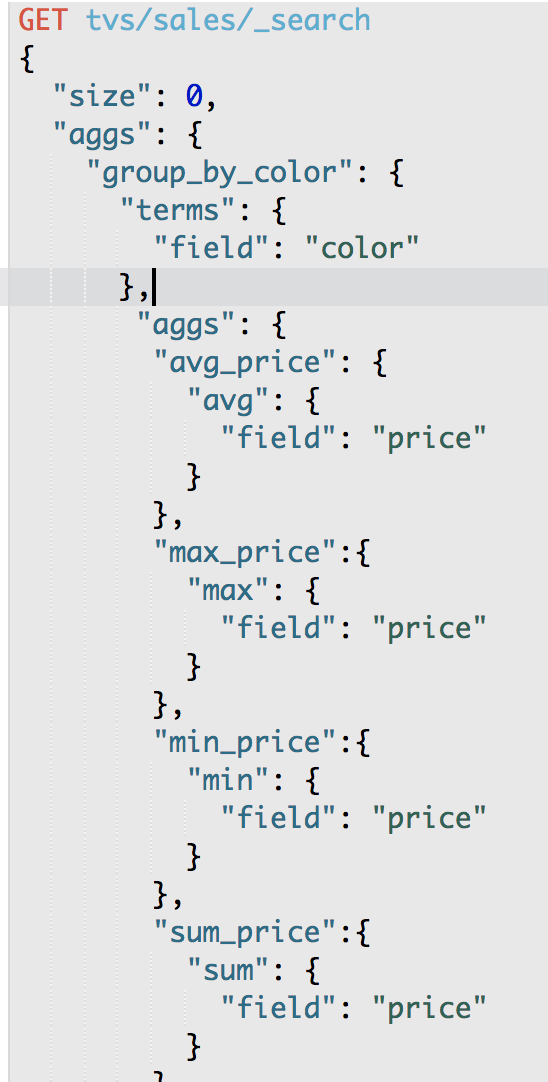
求总和，就可以拿到一个颜色下的所有电视的销售总额

{
"took": 16,
"timed_out": false,
"_shards": {
"total": 5,
"successful": 5,
"failed": 0
},
"hits": {
"total": 8,
"max_score": 0,
"hits": []
},
"aggregations": {
"group_by_color": {
"doc_count_error_upper_bound": 0,
"sum_other_doc_count": 0,
"buckets": [
{
"key": "红色",
"doc_count": 4,
"max_price": {
"value": 8000
},
"min_price": {
"value": 1000
},
"avg_price": {
"value": 3250
},
"sum_price": {
"value": 13000
}
},
{
"key": "绿色",
"doc_count": 2,
"max_price": {
"value": 3000
},
"min_price": {
"value":
}, 1200
"avg_price": {
"value": 2100
},
"sum_price": {
"value": 4200
}
},
{
"key": "蓝色",
"doc_count": 2,
"max_price": {
"value": 2500
},
"min_price": {
"value": 1500
},
"avg_price": {
"value": 2000
},
"sum_price": {
"value": 4000
}
}
]
}
}
}

第38节深入聚合数据分析_实战hitogram按价格区间统计电视销量和销售额

课程大纲

histogram：类似于terms，也是进行bucket分组操作，接收一个field，按照这个field的值的各个范围区间，进行bucket分组操作

"histogram":{
"field": "price",
"interval": 2000
},

interval：2000，划分范围，0~2000，2000~4000，4000~6000，6000~8000，8000~10000，buckets

去根据price的值，比如2500，看落在哪个区间内，比如2000~4000，此时就会将这条数据放入2000~4000对应的那个bucket中

bucket划分的方法，terms，将field值相同的数据划分到一个bucket中

bucket有了之后，一样的，去对每个bucket执行avg，count，sum，max，min，等各种metric操作，聚合分析

GET /tvs/sales/_search
{
"size" : 0,
"aggs":{
"price":{
"histogram":{
"field": "price",
"interval": 2000
},
"aggs":{
"revenue": {
"sum": {
"field" : "price"
}
}
}
}
}
}

{
"took": 13,
"timed_out": false,
"_shards": {
"total": 5,
"successful": 5,
"failed": 0
},
"hits": {
"total": 8,
"max_score": 0,
"hits": []
},
"aggregations": {
"group_by_price": {
"buckets": [
{
"key": 0,
"doc_count": 3,
"sum_price": {
"value": 3700
}
},
{
"key": 2000,
"doc_count": 4,
"sum_price": {
"value": 9500
}
},
{
"key": 4000,
"doc_count": 0,
"sum_price": {
"value": 0
}
},
{
"key": 6000,
"doc_count: {
"value":": 0,
"sum_price" 0
}
},
{
"key": 8000,
"doc_count": 1,
"sum_price": {
"value": 8000
}
}
]
}
}
}

第39节深入聚合数据分析_实战date hitogram之统计每月电视销量

课程大纲

bucket，分组操作，histogram，按照某个值指定的interval，划分一个一个的bucket

date histogram，按照我们指定的某个date类型的日期field，以及日期interval，按照一定的日期间隔，去划分bucket

date interval = 1m，

2017-01-01~2017-01-31，就是一个bucket
2017-02-01~2017-02-28，就是一个bucket

然后会去扫描每个数据的date field，判断date落在哪个bucket中，就将其放入那个bucket

2017-01-05，就将其放入2017-01-01~2017-01-31，就是一个bucket

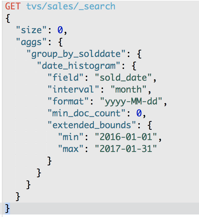
min_doc_count：即使某个日期interval，2017-01-01~2017-01-31中，一条数据都没有，那么这个区间也是要返回的，不然默认是会过滤掉这个区间的
extended_bounds，min，max：划分bucket的时候，会限定在这个起始日期，和截止日期内

GET /tvs/sales/_search
{
"size" : 0,
"aggs": {
"sales": {
"date_histogram": {
"field": "sold_date",
"interval": "month",
"format": "yyyy-MM-dd",
"min_doc_count" : 0,
"extended_bounds" : {
"min" : "2016-01-01",
"max" : "2017-12-31"
}
}
}
}
}

{
"took": 16,
"timed_out": false,
"_shards": {
"total": 5,
"successful": 5,
"failed": 0
},
"hits": {
"total": 8,
"max_score": 0,
"hits": []
},
"aggregations": {
"group_by_sold_date": {
"buckets": [
{
"key_as_string": "2016-01-01",
"key": 1451606400000,
"doc_count": 0
},
{
"key_as_string": "2016-02-01",
"key": 1454284800000,
"doc_count": 0
},
{
"key_as_string": "2016-03-01",
"key": 1456790400000,
"doc_count": 0
},
{
"key_as_string": "2016-04-01",
"key": 1459468800000,
"doc_count": 0
},
{
"key_as_string": "2016-05-01",
"key": 1462060800000,
"doc_count": 1
},
{
"key_as_string": "2016-06-01",
"key": 1464739200000,
"doc_count": 0
},
{
"key_as_string": "2016-07-01",
"key": 1467331200000,
"doc_count": 1
},
{
"key_as_strin
"key_as_string": "2016-09-01",
"key": 1472688000000,
"doc_count": 0
},g": "2016-08-01",
"key": 1470009600000,
"doc_count": 1
},
{
{
"key_as_string": "2016-10-01",
"key": 1475280000000,
"doc_count": 1
},
{
"key_as_string": "2016-11-01",
"key": 1477958400000,
"doc_count": 2
},
{
"key_as_string": "2016-12-01",
"key": 1480550400000,
"doc_count": 0
},
{
"key_as_string": "2017-01-01",
"key": 1483228800000,
"doc_count": 1
},
{
"key_as_string": "2017-02-01",
"key": 1485907200000,
"doc_count": 1
}
]
}
}
}

第40节深入聚合数据分析_下钻分析之统计每季度每个品牌的销售额

课程大纲

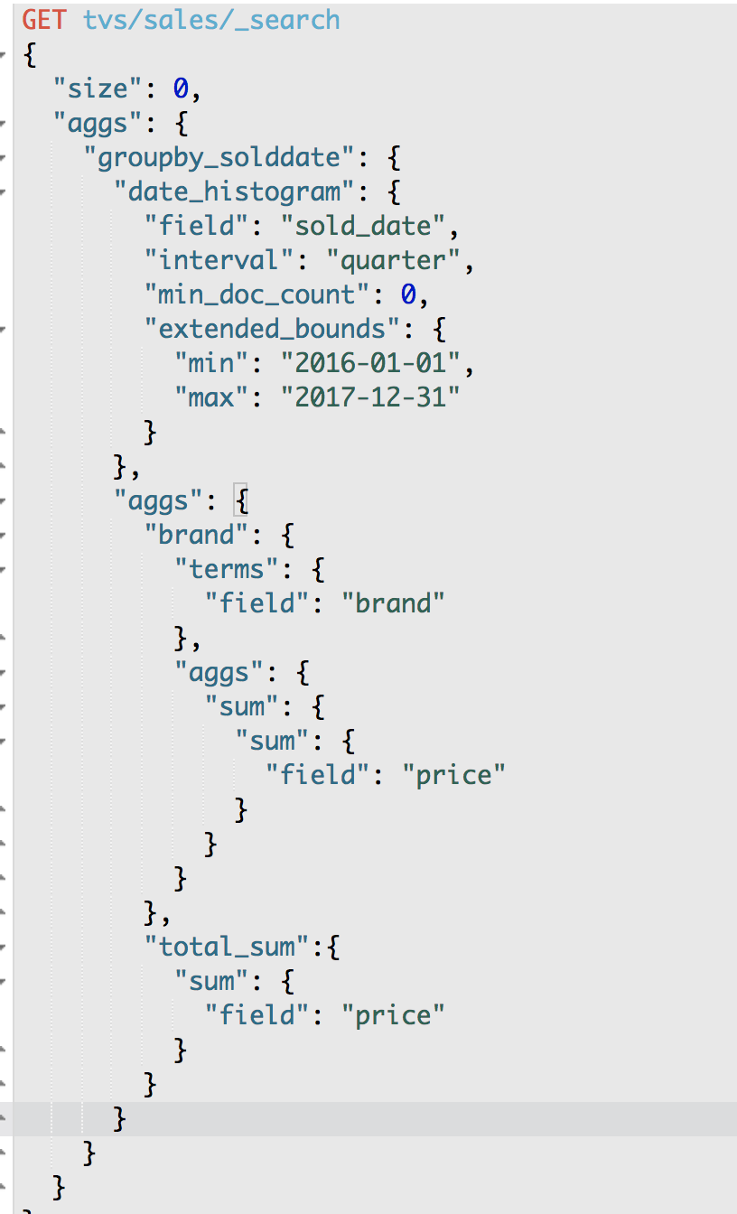
GET /tvs/sales/_search
{
"size": 0,
"aggs": {
"group_by_sold_date": {
"date_histogram": {
"field": "sold_date",
"interval": "quarter",     季度划分
"format": "yyyy-MM-dd",
"min_doc_count": 0,
"extended_bounds": {
"min": "2016-01-01",
"max": "2017-12-31"
}
},
"aggs": {
"group_by_brand": {
"terms": {
"field": "brand"
},
"aggs": {
"sum_price": {
"sum": {
"field": "price"
}
}
}
},
"total_sum_price": {
"sum": {
"field": "price"
}
}
}
}
}
}

{
"took": 10,
"timed_out": false,
"_shards": {
"total": 5,
"successful": 5,
"failed": 0
},
"hits": {
"total": 8,
"max_score": 0,
"hits": []
},
"aggregations": {
"group_by_sold_date": {
"buckets": [
{
"key_as_string": "2016-01-01",
"key": 1451606400000,
"doc_count": 0,
"total_sum_price": {
"value": 0
},
"group_by_brand": {
"doc_count_error_upper_bound": 0,
"sum_other_doc_count": 0,
"buckets": []
}
},
{
"key_as_string": "2016-04-01",
"key": 1459468800000,
"doc_count": 1,
"total_sum_price": {
"value": 3000
},
"group_by_brand": {
"doc_count_error_upper_bound": 0,
"sum_other_doc_count": 0,
"buckets": [
{
"key": "小米",
"doc_count": 1,
"sum_price": {
"value": 3000
}
}
]
}
},
{
"key_as_string": "2016-07-01",
"key": 1467331200000,
"doc_count": 2,
"total_sum_price": {
"value": 2700
},
"group_by_brand": {
"doc_count_error_upper_bound": 0,
"sum_other_doc_count": 0,
"buckets": [
{
"key": "TCL",
"doc_count": 2,
"sum_price": {
"value": 2700
}
}
]
}
},
{
"key_as_string": "2016-10-01",
"key": 1475280000000,
"doc_count": 3,
"total_sum_price": {
"value": 5000
},
"group_by_brand": {
"doc_count_error_upper_bound": 0,
"sum_other_doc_count": 0,
"buckets": [
{
"key": "长虹",
"doc_count": 3,
"sum_price": {
"value": 5000
}
}
]
}
},
{
"key_as_string": "2017-01-01",
"key": 1483228800000,
"doc_count": 2,
"total_sum_price": {
"value": 10500
},
"group_by_brand": {
"doc_count_error_upper_bound": 0,
"sum_other_doc_count": 0,
"buckets": [
{
"key": "三星",
"doc_count": 1,
"sum_price": {
"value": 8000
}
},
{
"key": "小米",
"doc_count": 1,
"sum_price": {
"value": 2500
}
}
]
}
},
{
"key_as_string": "2017-04-01",
"key": 1491004800000,
"doc_count": 0,
"total_sum_price": {
"value": 0
},
"group_by_brand": {
"doc_count_error_upper_bound": 0,
"sum_other_doc_count": 0,
"buckets": []
}
},
{
"key_as_string": "2017-07-01",
"key": 1498867200000,
"doc_count": 0,
"total_sum_price": {
"value": 0
},
"group_by_brand": {
"doc_count_error_upper_bound": 0,
"sum_other_doc_count": 0,
"buckets": []
}
},
{
"key_as_string": "2017-10-01",
"key": 1506816000000,
"doc_count": 0,
"total_sum_price": {
"value": 0
},
"group_by_brand": {
"doc_count_error_upper_bound": 0,
"sum_other_doc_count": 0,
"buckets": []
}
}
]
}
}
}

第41节深入聚合数据分析_搜索+聚合：统计指定品牌下每个颜色的销量

课程大纲

实际上来说，我们之前学习的搜索相关的知识，完全可以和聚合组合起来使用

select count(*)
from tvs.sales
where brand like "%长%"
group by price

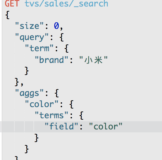
es aggregation，scope，任何的聚合，都必须在搜索出来的结果数据中之行，搜索结果，就是聚合分析操作的scope

GET /tvs/sales/_search
{
"size": 0,
"query": {
"term": {
"brand": {
"value": "小米"
}
}
},
"aggs": {
"group_by_color": {
"terms": {
"field": "color"
}
}
}
}

{
"took": 5,
"timed_out": false,
"_shards": {
"total": 5,
"successful": 5,
"failed": 0
},
"hits": {
"total": 2,
"max_score": 0,
"hits": []
},
"aggregations": {
"group_by_color": {
"doc_count_error_upper_bound": 0,
"sum_other_doc_count": 0,
"buckets": [
{
"key": "绿色",
"doc_count": 1
},
{
"key": "蓝色",
"doc_count": 1
}
]
}
}
}

第42节深入聚合数据分析_global bucket：单个品牌与所有品牌销量对比

课程大纲

aggregation，scope，一个聚合操作，必须在query的搜索结果范围内执行

出来两个结果，一个结果，是基于query搜索结果来聚合的; 一个结果，是对所有数据执行聚合的

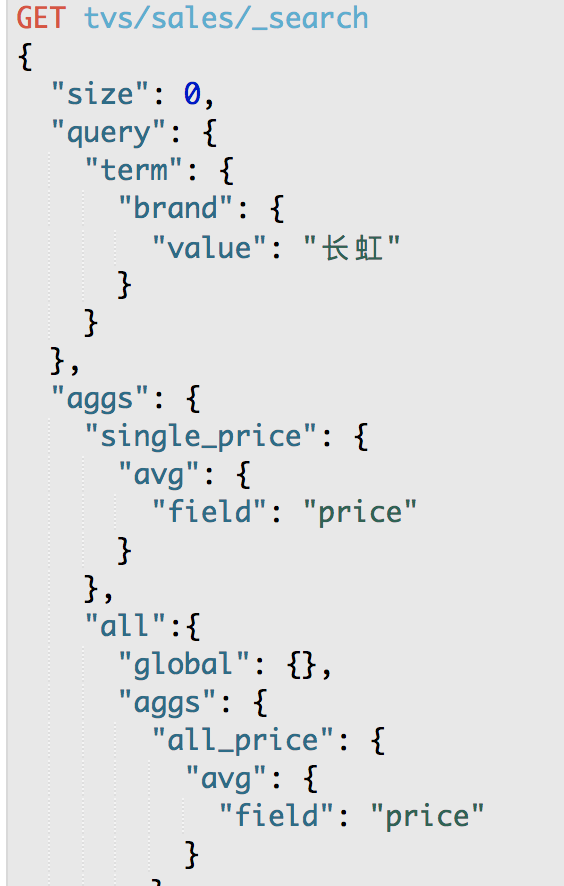
GET /tvs/sales/_search
{
"size": 0,
"query": {
"term": {
"brand": {
"value": "长虹"
}
}
},
"aggs": {
"single_brand_avg_price": {
"avg": {
"field": "price"
}
},
"all": {
"global": {},
"aggs": {
"all_brand_avg_price": {
"avg": {
"field": "price"
}
}
}
}
}
}

global：就是global bucket，就是将所有数据纳入聚合的scope，而不管之前的query

{
"took": 4,
"timed_out": false,
"_shards": {
"total": 5,
"successful": 5,
"failed": 0
},
"hits": {
"total": 3,
"max_score": 0,
"hits": []
},
"aggregations": {
"all": {
"doc_count": 8,
"all_brand_avg_price": {
"value": 2650
}
},
"single_brand_avg_price": {
"value": 1666.6666666666667
}
}
}

single_brand_avg_price：就是针对query搜索结果，执行的，拿到的，就是长虹品牌的平均价格
all.all_brand_avg_price：拿到所有品牌的平均价格

第43节深入聚合数据分析_过滤+聚合：统计价格大于1200的电视平均价格

课程大纲

搜索+聚合
过滤+聚合

GET /tvs/sales/_search
{
"size": 0,
"query": {
"constant_score": {
"filter": {
"range": {
"price": {
"gte": 1200
}
}
}
}
},
"aggs": {
"avg_price": {
"avg": {
"field": "price"
}
}
}
}

{
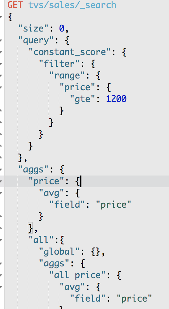
"took": 41,
"timed_out": false,
"_shards": {
"total": 5,
"successful": 5,
"failed": 0
},
"hits": {
"total": 7,
"max_score": 0,
"hits": []
},
"aggregations": {
"avg_price": {
"value": 2885.714285714286
}
}
}

第44节深入聚合数据分析_bucket filter：统计牌品最近一个月的平均价格

课程大纲

GET /tvs/sales/_search
{
"size": 0,
"query": {
"term": {
"brand": {
"value": "长虹"
}
}
},
"aggs": {
"recent_150d": {
"filter": {
"range": {
"sold_date": {
"gte": "now-150d"
}
}
},
"aggs": {
"recent_150d_avg_price": {
"avg": {
"field": "price"
}
}
}
},
"recent_140d": {
"filter": {
"range": {
"sold_date": {
"gte": "now-140d"
}
}
},
"aggs": {
"recent_140d_avg_price": {
"avg": {
"field": "price"
}
}
}
},
"recent_130d": {
"filter": {
"range": {
"sold_date": {
"gte": "now-130d"
}
}
},
"aggs": {
"recent_130d_avg_price": {
"avg": {
"field": "price"
}
}
}
}
}
}

aggs.filter，针对的是聚合去做的

如果放query里面的filter，是全局的，会对所有的数据都有影响

但是，如果，比如说，你要统计，长虹电视，最近1个月的平均值; 最近3个月的平均值; 最近6个月的平均值

bucket filter：对不同的bucket下的aggs，进行filter

第45节深入聚合数据分析_排序：按每种颜色的平均销售额降序排序

课程大纲

之前的话，排序，是按照每个bucket的doc_count降序来排的

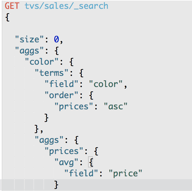
但是假如说，我们现在统计出来每个颜色的电视的销售额，需要按照销售额降序排序？？？？

GET /tvs/sales/_search
{
"size": 0,
"aggs": {
"group_by_color": {
"terms": {
"field": "color"
},
"aggs": {
"avg_price": {
"avg": {
"field": "price"
}
}
}
}
}
}

{
"took": 2,
"timed_out": false,
"_shards": {
"total": 5,
"successful": 5,
"failed": 0
},
"hits": {
"total": 8,
"max_score": 0,
"hits": []
},
"aggregations": {
"group_by_color": {
"doc_count_error_upper_bound": 0,
"sum_other_doc_count": 0,
"buckets": [
{
"key": "红色",
"doc_count": 4,
"avg_price": {
"value": 3250
}
},
{
"key": "绿色",
"doc_count": 2,
"avg_price": {
"value": 2100
}
},
{
"key": "蓝色",
"doc_count": 2,
"avg_price": {
"value": 2000
}
}
]
}
}
}

GET /tvs/sales/_search
{
"size": 0,
"aggs": {
"group_by_color": {
"terms": {
"field": "color",
"order": {
"avg_price": "asc"
}
},
"aggs": {
"avg_price": {
"avg": {
"field": "price"
}
}
}
}
}
}

第46节深入聚合数据分析_颜色+品牌下钻分析时按最深层metric进行排序

课程大纲

GET /tvs/sales/_search
{
"size": 0,
"aggs": {
"group_by_color": {
"terms": {
"field": "color"
},
"aggs": {
"group_by_brand": {
"terms": {
"field": "brand",
"order": {
"avg_price": "desc"
}
},
"aggs": {
"avg_price": {
"avg": {
"field": "price"
}
}
}
}
}
}
}
}

{
"took": 4,
"timed_out": false,
"_shards": {
"total": 5,
"successful": 5,
"failed": 0
},
"hits": {
"total": 8,
"max_score": 0,
"hits": []
},
"aggregations": {
"group_by_color": {
"doc_count_error_upper_bound": 0,
"sum_other_doc_count": 0,
"buckets": [
{
"key": "红色",
"doc_count": 4,
"group_by_brand": {
"doc_count_error_upper_bound": 0,
"sum_other_doc_count": 0,
"buckets": [
{
"key": "三星",
"doc_count": 1,
"avg_price": {
"value": 8000
}
},
{
"key": "长虹",
"doc_count": 3,
"avg_price": {
"value": 1666.6666666666667
}
}
]
}
},
{
"key": "绿色",
"doc_count": 2,
"group_by_brand": {
"doc_count_error_upper_bound": 0,
"sum_other_doc_count": 0,
"buckets": [
{
"key": "小米",
"doc_count": 1,
"avg_price": {
"value": 3000
}
},
{
"key": "TCL",
"doc_count": 1,
"avg_price": {
"value": 1200
}
}
]
}
},
{
"key": "蓝色",
"doc_count": 2,
"group_by_brand": {
"doc_count_error_upper_bound": 0,
"sum_other_doc_count": 0,
"buckets": [
{
"key": "小米",
"doc_count": 1,
"avg_price": {
"value": 2500
}
},
{
"key": "TCL",
"doc_count": 1,
"avg_price": {
"value": 1500
}
}
]
}
}
]
}
}
}

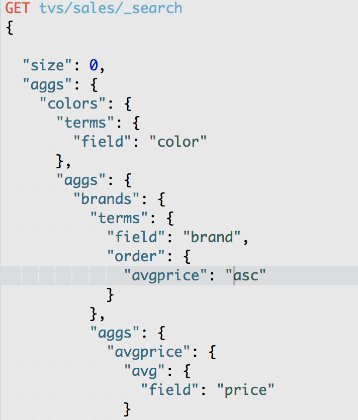
在最深层的bucket中做order by！！！