【pytorch】改造resnet为全卷积神经网络以适应不同大小的输入

为什么resnet的输入是一定的？

因为resnet最后有一个全连接层。正是因为这个全连接层导致了输入的图像的大小必须是固定的。

输入为固定的大小有什么局限性？

原始的resnet在imagenet数据集上都会将图像缩放成224×224的大小，但这么做会有一些局限性：

（1）当目标对象占据图像中的位置很小时，对图像进行缩放将导致图像中的对象进一步缩小，图像可能不会正确被分类

（2）当图像不是正方形或对象不位于图像的中心处，缩放将导致图像变形

（3）如果使用滑动窗口法去寻找目标对象，这种操作是昂贵的

如何修改resnet使其适应不同大小的输入？

（1）自定义一个自己网络类，但是需要继承models.ResNet

（2）将自适应平均池化替换成普通的平均池化

（3）将全连接层替换成卷积层

相关代码：

import torch
import torch.nn as nn
from torchvision import models
import torchvision.transforms as transforms
from torch.hub import load_state_dict_from_url

from PIL import Image
import cv2
import numpy as np
from matplotlib import pyplot as plt

class FullyConvolutionalResnet18(models.ResNet):
    def __init__(self, num_classes=1000, pretrained=False, **kwargs):

        # Start with standard resnet18 defined here
        super().__init__(block = models.resnet.BasicBlock, layers = [2, 2, 2, 2], num_classes = num_classes, **kwargs)
        if pretrained:
            state_dict = load_state_dict_from_url( models.resnet.model_urls["resnet18"], progress=True)
            self.load_state_dict(state_dict)

        # Replace AdaptiveAvgPool2d with standard AvgPool2d
        self.avgpool = nn.AvgPool2d((7, 7))

        # Convert the original fc layer to a convolutional layer.
        self.last_conv = torch.nn.Conv2d( in_channels = self.fc.in_features, out_channels = num_classes, kernel_size = 1)
        self.last_conv.weight.data.copy_( self.fc.weight.data.view ( *self.fc.weight.data.shape, 1, 1))
        self.last_conv.bias.data.copy_ (self.fc.bias.data)

    # Reimplementing forward pass.
    def _forward_impl(self, x):
        # Standard forward for resnet18
        x = self.conv1(x)
        x = self.bn1(x)
        x = self.relu(x)
        x = self.maxpool(x)

        x = self.layer1(x)
        x = self.layer2(x)
        x = self.layer3(x)
        x = self.layer4(x)
        x = self.avgpool(x)

        # Notice, there is no forward pass
        # through the original fully connected layer.
        # Instead, we forward pass through the last conv layer
        x = self.last_conv(x)
        return x

需要注意的是我们将全连接层的参数拷贝到自己定义的卷积层中去了。

看一下网络结构，主要是关注网络的最后：

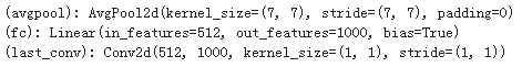
我们将self.avgpool替换成了AvgPool2d，而全连接层虽然还在网络中，但是在前向传播时我们并没有用到 。

现在我们有这么一张图像：

图像大小为：(387, 1024, 3)。而且目标对象骆驼是位于图像的右下角的。

我们就以这张图片看一下是怎么使用的。

with open('imagenet_classes.txt') as f:
    labels = [line.strip() for line in f.readlines()]

# Read image
original_image = cv2.imread('camel.jpg')# Convert original image to RGB format
image = cv2.cvtColor(original_image, cv2.COLOR_BGR2RGB)

# Transform input image
# 1. Convert to Tensor
# 2. Subtract mean
# 3. Divide by standard deviation

transform = transforms.Compose([
              transforms.ToTensor(), #Convert image to tensor.
              transforms.Normalize(
              mean=[0.485, 0.456, 0.406],   # Subtract mean
              std=[0.229, 0.224, 0.225]     # Divide by standard deviation
              )])

image = transform(image)
image = image.unsqueeze(0)
# Load modified resnet18 model with pretrained ImageNet weights
model = fcresnet18.FullyConvolutionalResnet18(pretrained=True).eval()
print(model)
with torch.no_grad():
    # Perform inference.
    # Instead of a 1x1000 vector, we will get a
    # 1x1000xnxm output ( i.e. a probabibility map
    # of size n x m for each 1000 class,
    # where n and m depend on the size of the image.)
    preds = model(image)
    preds = torch.softmax(preds, dim=1)

    print('Response map shape : ', preds.shape)

    # Find the class with the maximum score in the n x m output map
    pred, class_idx = torch.max(preds, dim=1)
    print(class_idx)

    row_max, row_idx = torch.max(pred, dim=1)
    col_max, col_idx = torch.max(row_max, dim=1)
    predicted_class = class_idx[0, row_idx[0, col_idx], col_idx]

    # Print top predicted class
    print('Predicted Class : ', labels[predicted_class], predicted_class)

说明：imagenet_classes.txt中是标签信息。在数据增强时，并没有将图像重新调整大小。用opencv读取的图片的格式为BGR，我们需要将其转换为pytorch的格式：RGB。同时需要使用unsqueeze(0)增加一个维度，变成[batchsize,channel,height,width]。看一下avgpool和last_conv的输出的维度：

我们使用torchsummary库来进行每一层输出的查看：

device = torch.device("cuda" if torch.cuda.is_available() else "cpu")
model.to(device)
from torchsummary import summary
summary(model, (3, 387, 1024))

结果：

----------------------------------------------------------------
        Layer (type)               Output Shape         Param #
================================================================
            Conv2d-1         [-1, 64, 194, 512]           9,408
       BatchNorm2d-2         [-1, 64, 194, 512]             128
              ReLU-3         [-1, 64, 194, 512]               0
         MaxPool2d-4          [-1, 64, 97, 256]               0
            Conv2d-5          [-1, 64, 97, 256]          36,864
       BatchNorm2d-6          [-1, 64, 97, 256]             128
              ReLU-7          [-1, 64, 97, 256]               0
            Conv2d-8          [-1, 64, 97, 256]          36,864
       BatchNorm2d-9          [-1, 64, 97, 256]             128
             ReLU-10          [-1, 64, 97, 256]               0
       BasicBlock-11          [-1, 64, 97, 256]               0
           Conv2d-12          [-1, 64, 97, 256]          36,864
      BatchNorm2d-13          [-1, 64, 97, 256]             128
             ReLU-14          [-1, 64, 97, 256]               0
           Conv2d-15          [-1, 64, 97, 256]          36,864
      BatchNorm2d-16          [-1, 64, 97, 256]             128
             ReLU-17          [-1, 64, 97, 256]               0
       BasicBlock-18          [-1, 64, 97, 256]               0
           Conv2d-19         [-1, 128, 49, 128]          73,728
      BatchNorm2d-20         [-1, 128, 49, 128]             256
             ReLU-21         [-1, 128, 49, 128]               0
           Conv2d-22         [-1, 128, 49, 128]         147,456
      BatchNorm2d-23         [-1, 128, 49, 128]             256
           Conv2d-24         [-1, 128, 49, 128]           8,192
      BatchNorm2d-25         [-1, 128, 49, 128]             256
             ReLU-26         [-1, 128, 49, 128]               0
       BasicBlock-27         [-1, 128, 49, 128]               0
           Conv2d-28         [-1, 128, 49, 128]         147,456
      BatchNorm2d-29         [-1, 128, 49, 128]             256
             ReLU-30         [-1, 128, 49, 128]               0
           Conv2d-31         [-1, 128, 49, 128]         147,456
      BatchNorm2d-32         [-1, 128, 49, 128]             256
             ReLU-33         [-1, 128, 49, 128]               0
       BasicBlock-34         [-1, 128, 49, 128]               0
           Conv2d-35          [-1, 256, 25, 64]         294,912
      BatchNorm2d-36          [-1, 256, 25, 64]             512
             ReLU-37          [-1, 256, 25, 64]               0
           Conv2d-38          [-1, 256, 25, 64]         589,824
      BatchNorm2d-39          [-1, 256, 25, 64]             512
           Conv2d-40          [-1, 256, 25, 64]          32,768
      BatchNorm2d-41          [-1, 256, 25, 64]             512
             ReLU-42          [-1, 256, 25, 64]               0
       BasicBlock-43          [-1, 256, 25, 64]               0
           Conv2d-44          [-1, 256, 25, 64]         589,824
      BatchNorm2d-45          [-1, 256, 25, 64]             512
             ReLU-46          [-1, 256, 25, 64]               0
           Conv2d-47          [-1, 256, 25, 64]         589,824
      BatchNorm2d-48          [-1, 256, 25, 64]             512
             ReLU-49          [-1, 256, 25, 64]               0
       BasicBlock-50          [-1, 256, 25, 64]               0
           Conv2d-51          [-1, 512, 13, 32]       1,179,648
      BatchNorm2d-52          [-1, 512, 13, 32]           1,024
             ReLU-53          [-1, 512, 13, 32]               0
           Conv2d-54          [-1, 512, 13, 32]       2,359,296
      BatchNorm2d-55          [-1, 512, 13, 32]           1,024
           Conv2d-56          [-1, 512, 13, 32]         131,072
      BatchNorm2d-57          [-1, 512, 13, 32]           1,024
             ReLU-58          [-1, 512, 13, 32]               0
       BasicBlock-59          [-1, 512, 13, 32]               0
           Conv2d-60          [-1, 512, 13, 32]       2,359,296
      BatchNorm2d-61          [-1, 512, 13, 32]           1,024
             ReLU-62          [-1, 512, 13, 32]               0
           Conv2d-63          [-1, 512, 13, 32]       2,359,296
      BatchNorm2d-64          [-1, 512, 13, 32]           1,024
             ReLU-65          [-1, 512, 13, 32]               0
       BasicBlock-66          [-1, 512, 13, 32]               0
        AvgPool2d-67            [-1, 512, 1, 4]               0
           Conv2d-68           [-1, 1000, 1, 4]         513,000
================================================================
Total params: 11,689,512
Trainable params: 11,689,512
Non-trainable params: 0
----------------------------------------------------------------
Input size (MB): 4.54
Forward/backward pass size (MB): 501.42
Params size (MB): 44.59
Estimated Total Size (MB): 550.55
----------------------------------------------------------------

最后是看一下预测的结果：

Response map shape :  torch.Size([1, 1000, 1, 4])
tensor([[[978, 980, 970, 354]]])
Predicted Class :  Arabian camel, dromedary, Camelus dromedarius tensor([354])

与imagenet_classes.txt中对应（索引下标是从0开始的）

可视化关注点：

from google.colab.patches import cv2_imshow
# Find the n x m score map for the predicted class
score_map = preds[0, predicted_class, :, :].cpu().numpy()
score_map = score_map[0]

# Resize score map to the original image size
score_map = cv2.resize(score_map, (original_image.shape[1], original_image.shape[0]))

# Binarize score map
_, score_map_for_contours = cv2.threshold(score_map, 0.25, 1, type=cv2.THRESH_BINARY)
score_map_for_contours = score_map_for_contours.astype(np.uint8).copy()

# Find the countour of the binary blob
contours, _ = cv2.findContours(score_map_for_contours, mode=cv2.RETR_EXTERNAL, method=cv2.CHAIN_APPROX_SIMPLE)

# Find bounding box around the object.
rect = cv2.boundingRect(contours[0])
# Apply score map as a mask to original image
score_map = score_map - np.min(score_map[:])
score_map = score_map / np.max(score_map[:])
score_map = cv2.cvtColor(score_map, cv2.COLOR_GRAY2BGR)
masked_image = (original_image * score_map).astype(np.uint8)

# Display bounding box
cv2.rectangle(masked_image, rect[:2], (rect[0] + rect[2], rect[1] + rect[3]), (0, 0, 255), 2)

# Display images
#cv2.imshow("Original Image", original_image)
#cv2.imshow("activations_and_bbox", masked_image)
cv2_imshow(original_image)
cv2_imshow(masked_image)
cv2.waitKey(0)

在谷歌colab中ipynb要使用：from google.colab.patches import cv2_imshow

而不能使用opencv自带的cv2.show()

结果：

参考：https://www.learnopencv.com/cnn-receptive-field-computation-using-backprop/?ck_subscriber_id=503149816