Tensorflow Probability Distributions 简介

摘要：Tensorflow Distributions提供了两类抽象：distributions和bijectors。distributions提供了一系列具备快速、数值稳定的采样、对数概率计算以及其他统计特征计算方法的概率分布。bijectors提供了一系列针对distribution的可组合的确定性变换。

1、Distributions

1.1 methods

一个distribution至少实现以下方法：sample、log_prob、batch_shape_tensor、event_shape_tensor；同时也实现了一些其他方法，例如：cdf、survival_function、quantile、mean、variance、entropy等；Distribution基类实现了给定log_prob计算prob、给定log_cdf计算log_survival_fn的方法。

1.2 shape semantics

将一个tensor的形状分为三个部分：sample shape、batch shape、event shape。

sample shape：描述从给定概率分布上独立同分布的采样形状；

batch shape：描述从概率分布上独立、非同分布的采样形状，也即，我们可以指定一组参数不同的相同分布，batch shape通常用来为机器学习中一个batch的样本每个样本指定一个分布；

event shape：描述从概率分布上单次采样的形状；

1.3 sampling

reparameterization：distributions拥有一个reparameterization属性，这个属性表明了自动化微分和采样之间的关系。目前包括两种：“fully reparameterized” 和 “not reparameterized”。

fully reparameterized：例如，对于分布dist = Normal(loc, scale)，采样y = dist.sample()的内部过程为x = tf.random_normal([]); y = scale * x + loc. 样本y是reparameterized的，因为它是参数loc、scale及无参数样本x的光滑函数。

not reparameterized：例如，gamma分布使用接收-拒绝的方式进行采样，是参数的非光滑函数。

end to end automatic differentiation：通过与tensorflow结合，一个fully reparameterized的分布可以进行端到端的自动微分。例如，要最小化分布Y的期望损失E [φ(Y)]，可以使用蒙特卡洛近似的方法最小化

这使得我们可以使用S_N作为期望损失的估计，还可以使用Δ_λS_N作为梯度Δ_λE [φ(Y)]的估计，其中λ是分布Y的参数。

1.4 high order distributions

 TransformedDistribution：对一个基分布执行一个可逆可微分转换即可得到一个TransformedDistribution。例如，可以从一个Exponential分布得到一个标准Gumbel分布：

standard_gumbel = tfd.TransformedDistribution(
    distribution=tfd.Exponential(rate=1.),
    bijector=tfb.Chain([
        tfb.Affine(
            scale_identity_multiplier=-1.,
            event_ndims=0),
        tfb.Invert(tfb.Exp()),
    ]))
standard_gumbel.batch_shape  # ==> []
standard_gumbel.event_shape  # ==> []

基于gumbel分布，可以构建一个Gumbel-Softmax(Concrete)分布：

alpha = tf.stack([
    tf.fill([28 * 28], 2.),
    tf.ones(28 * 28)])

concrete_pixel = tfd.TransformedDistribution(
    distribution=standard_gumbel,
    bijector=tfb.Chain([
        tfb.Sigmoid(),
        tfb.Affine(shift=tf.log(alpha)),
    ]),
    batch_shape=[2, 28 * 28])
concrete_pixel.batch_shape  # ==> [2, 784]
concrete_pixel.event_shape  # ==> []

Independent：对batch shape和event shape进行转换。例如：

image_dist = tfd.TransformedDistribution(
    distribution=tfd.Independent(concrete_pixel),
    bijector=tfb.Reshape(
        event_shape_out=[28, 28, 1],
        event_shape_in=[28 * 28]))
image_dist.batch_shape  # ==> [2]
image_dist.event_shape  # ==> [28, 28, 1]

Mixture：定义了由若干分布组合成的新的分布，例如：

image_mixture = tfd.MixtureSameFamily(
    mixture_distribution=tfd.Categorical(
        probs=[0.2, 0.8]),
    components_distribution=image_dist)
image_mixture.batch_shape  # ==> []
image_mixture.event_shape  # ==> [28, 28, 1]

1.5 distribution functionals

functional以一个分布作为输入，输出一个标量，例如：entropy、cross entropy、mutual information、kl距离等。

p = tfd.Normal(loc=0., scale=1.)
q = tfd.Normal(loc=-1., scale=2.)
xent = p.cross_entropy(q)
kl = p.kl_divergence(q)
# ==> xent - p.entropy()

2、Bijectors

2.1 definition

Bijector API提供了针对distribution的可微分双向映射（differentialble, bijective map, diffeomorphism）转换接口。给定随机变量X和一个diffeomorphism F，可以定义一个新的随机变量Y，Y的密度可由下式计算：

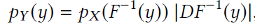
其中DF^-1是F的Jacobian的逆。（参考：https://zhuanlan.zhihu.com/p/100287713）

每个bijector子类都对应一个F，TransformedDistribution自动计算Y=F(X)的密度。bijector使得我们可以利用已有的分布构建许多其他分布。

bijector主要包含以下三个函数：

forward：实现x → F (x)，TransformedDistribution.sample函数使用该函数将一个tensor转换为另一个tensor；

inverse：forward的逆变换，实现y → F^-1(y)，TransformedDistribution.log_prob使用该函数计算对数概率（上式）；

inverse_log_det_jacobian：计算log |DF⁻¹(y)|，TransformedDistribution.log_prob使用该函数计算对数概率（上式）；

通过使用bijectors，TransformedDistribution可以自动高效地实现sample、log_prob、prob，对于具有恒定Jacobian的bijector，TransformedDistribution自动实现一些基础统计量，如mean、variance、entropy等。

以下实现了对Laplace的放射变换：

vector_laplace = tfd.TransformedDistribution(
    distribution=tfd.Laplace(loc=0., scale=1.),
    bijector=tfb.Affine(
        shift=tf.Variable(tf.zeros(d)),
        scale_tril=tfd.fill_triangular(
            tf.Variable(tf.ones(d * (d + 1) / 2)))),
    event_shape=[d])

由于tf.Variables，该分布是可学习的。

2.2 composability

bijectors可以构成高阶bijectors，例如Chain、Invert。

chain bijector可以构建一系列丰富的分布，例如创建一个多变量logit-Normal分布：

matrix_logit_mvn =
tfd.TransformedDistribution(
    distribution=tfd.Normal(0., 1.),
    bijector=tfb.Chain([
        tfb.Reshape([d, d]),
        tfb.SoftmaxCentered(),
        tfb.Affine(scale_diag=diag),
    ]),
    event_shape=[d * d])

Invert可以通过交换inverse和forward函数，高效地将bijectors数量翻倍，例如：

softminus_gamma = tfd.TransformedDistribution(
    distribution=tfd.Gamma(
        concentration=alpha,
        rate=beta),
    bijector=tfb.Invert(tfb.Softplus()))

2.3 caching

bijector自动缓存操作的输入输出对，包括log det jacobian。caching的意义时，当inverse计算很慢或数值不稳定或难以实现时，可以高效的执行inverse操作。当计算采样结果的概率是，缓存被触发。如果q(x)是x=f(ε)的密度，且ε~r，那么caching可以降低计算q(xi)的计算成本：

caching机制也可用来进行高效地重要性采样（importance sampling）：

3、 应用

3.1 核密度估计（KDE）

例如，可以通过以下代码构建一个由n个mvn_diag分布作为kernel的混合高斯模型，其中每个kernel的权重为1/n。注意，此时Independent会对分布的shape进行重定义（reinterpret），tfd.Normal(loc=x, scale=1.)创建了一个batch_shape = n*d, event_shape = []的分布，对其Independent之后，变为batch_shape = n, event_shape = d的分布。

Independent文档：https://www.tensorflow.org/probability/api_docs/python/tfp/distributions/Independent?hl=zh-cn

f = lambda x: tfd.Independent(tfd.Normal(
    loc=x, scale=1.))
n = x.shape[0].value
kde = tfd.MixtureSameFamily(
    mixture_distribution=tfd.Categorical(
        probs=[1 / n] * n),
    components_distribution=f(x))

3.2 变分自编码器（VAE）

论文：https://arxiv.org/pdf/1312.6114.pdf

博客：https://spaces.ac.cn/archives/5253

def make_encoder(x, z_size=8):
    net = make_nn(x, z_size * 2)

return tfd.MultivariateNormalDiag(
    loc=net[..., :z_size],
    scale=tf.nn.softplus(net[..., z_size:])))

def make_decoder(z, x_shape=(28, 28, 1)):
    net = make_nn(z, tf.reduce_prod(x_shape))

logits = tf.reshape(
    net, tf.concat([[-1], x_shape], axis=0))
return tfd.Independent(tfd.Bernoulli(logits))

def make_prior(z_size=8, dtype=tf.float32):
    return tfd.MultivariateNormalDiag(
        loc=tf.zeros(z_size, dtype)))

    def make_nn(x, out_size, hidden_size=(128, 64)):
        net = tf.flatten(x)

    for h in hidden_size:
        net = tf.layers.dense(
            net, h, activation=tf.nn.relu)
    return tf.layers.dense(net, out_size)

3.3 Edward概率编程

tfd是Edward的后端。以下代码实现一个随机循环神经网络（stochastic rnn），其隐藏状态是随机的。

stochastic rnn论文：https://arxiv.org/pdf/1411.7610.pdf

from edward.models import Normal

z = x = []
z[0] = Normal(loc=tf.zeros(K), scale=tf.ones(K))
h = tf.layers.dense(
    z[0], 512, activation=tf.nn.relu)
loc = tf.layers.dense(h, D, activation=None)
x[0] = Normal(loc=loc, scale=0.5)
for t in range(1, T):
    inputs = tf.concat([z[t - 1], x[t - 1]], 0)
    loc = tf.layers.dense(
        inputs, K, activation=tf.tanh)
    z[t] = Normal(loc=loc, scale=0.1)
    h = tf.layers.dense(
        z[t], 512, activation=tf.nn.relu)
    loc = tf.layers.dense(h, D, activation=None)
    x[t] = Normal(loc=loc, scale=0.5)