Pandas -- Merge,join and concatenate

Merge, join, and concatenate

pandas provides various facilities for easily combining together Series, DataFrame, and Panel objects with various kinds of set logic for the indexes and relational algebra functionality in the case of join / merge-type operations.

Concatenating objects

The concat function (in the main pandas namespace) does all of the heavy lifting of performing concatenation operations along an axis while performing optional set logic (union or intersection) of the indexes (if any) on the other axes. Note that I say “if any” because there is only a single possible axis of concatenation for Series.

Before diving into all of the details of concat and what it can do, here is a simple example:

In [1]: df1 = pd.DataFrame({'A': ['A0', 'A1', 'A2', 'A3'],
   ...:                     'B': ['B0', 'B1', 'B2', 'B3'],
   ...:                     'C': ['C0', 'C1', 'C2', 'C3'],
   ...:                     'D': ['D0', 'D1', 'D2', 'D3']},
   ...:                     index=[0, 1, 2, 3])
   ...: 

In [2]: df2 = pd.DataFrame({'A': ['A4', 'A5', 'A6', 'A7'],
   ...:                     'B': ['B4', 'B5', 'B6', 'B7'],
   ...:                     'C': ['C4', 'C5', 'C6', 'C7'],
   ...:                     'D': ['D4', 'D5', 'D6', 'D7']},
   ...:                      index=[4, 5, 6, 7])
   ...: 

In [3]: df3 = pd.DataFrame({'A': ['A8', 'A9', 'A10', 'A11'],
   ...:                     'B': ['B8', 'B9', 'B10', 'B11'],
   ...:                     'C': ['C8', 'C9', 'C10', 'C11'],
   ...:                     'D': ['D8', 'D9', 'D10', 'D11']},
   ...:                     index=[8, 9, 10, 11])
   ...: 

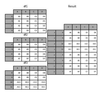
In [4]: frames = [df1, df2, df3]

In [5]: result = pd.concat(frames)

　　

 

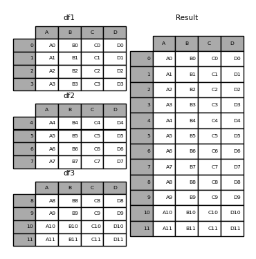
Like its sibling function on ndarrays, numpy.concatenate, pandas.concat takes a list or dict of homogeneously-typed objects and concatenates them with some configurable handling of “what to do with the other axes”:

pd.concat(objs, axis=0, join='outer', join_axes=None, ignore_index=False,
          keys=None, levels=None, names=None, verify_integrity=False,
          copy=True)

　　

• objs : a sequence or mapping of Series, DataFrame, or Panel objects. If a dict is passed, the sorted keys will be used as the keys argument, unless it is passed, in which case the values will be selected (see below). Any None objects will be dropped silently unless they are all None in which case a ValueError will be raised.
• axis : {0, 1, ...}, default 0. The axis to concatenate along.
• join : {‘inner’, ‘outer’}, default ‘outer’. How to handle indexes on other axis(es). Outer for union and inner for intersection.
• ignore_index : boolean, default False. If True, do not use the index values on the concatenation axis. The resulting axis will be labeled 0, ..., n - 1. This is useful if you are concatenating objects where the concatenation axis does not have meaningful indexing information. Note the index values on the other axes are still respected in the join.
• join_axes : list of Index objects. Specific indexes to use for the other n - 1 axes instead of performing inner/outer set logic.
• keys : sequence, default None. Construct hierarchical index using the passed keys as the outermost level. If multiple levels passed, should contain tuples.
• levels : list of sequences, default None. Specific levels (unique values) to use for constructing a MultiIndex. Otherwise they will be inferred from the keys.
• names : list, default None. Names for the levels in the resulting hierarchical index.
• verify_integrity : boolean, default False. Check whether the new concatenated axis contains duplicates. This can be very expensive relative to the actual data concatenation.
• copy : boolean, default True. If False, do not copy data unnecessarily.

Without a little bit of context and example many of these arguments don’t make much sense. Let’s take the above example. Suppose we wanted to associate specific keys with each of the pieces of the chopped up DataFrame. We can do this using the keys argument:

In [6]: result = pd.concat(frames, keys=['x', 'y', 'z'])

　　

 

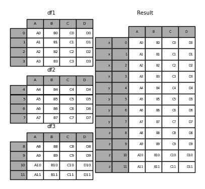
As you can see (if you’ve read the rest of the documentation), the resulting object’s index has a hierarchical index. This means that we can now do stuff like select out each chunk by key:

In [7]: result.ix['y']
Out[7]:
    A   B   C   D
4  A4  B4  C4  D4
5  A5  B5  C5  D5
6  A6  B6  C6  D6
7  A7  B7  C7  D7

　　

It’s not a stretch to see how this can be very useful. More detail on this functionality below.

Note

It is worth noting however, that concat (and therefore append) makes a full copy of the data, and that constantly reusing this function can create a significant performance hit. If you need to use the operation over several datasets, use a list comprehension.

frames = [ process_your_file(f) for f in files ]
result = pd.concat(frames)

　　

Set logic on the other axes

When gluing together multiple DataFrames (or Panels or...), for example, you have a choice of how to handle the other axes (other than the one being concatenated). This can be done in three ways:

• Take the (sorted) union of them all, join='outer'. This is the default option as it results in zero information loss.
• Take the intersection, join='inner'.
• Use a specific index (in the case of DataFrame) or indexes (in the case of Panel or future higher dimensional objects), i.e. the join_axes argument

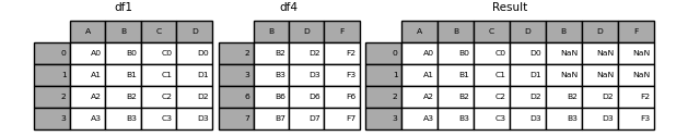
Here is a example of each of these methods. First, the default join='outer' behavior:

In [8]: df4 = pd.DataFrame({'B': ['B2', 'B3', 'B6', 'B7'],
   ...:                  'D': ['D2', 'D3', 'D6', 'D7'],
   ...:                  'F': ['F2', 'F3', 'F6', 'F7']},
   ...:                 index=[2, 3, 6, 7])
   ...: 

In [9]: result = pd.concat([df1, df4], axis=1)

　　

 

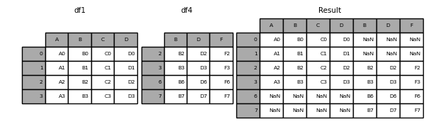
Note that the row indexes have been unioned and sorted. Here is the same thing with join='inner':

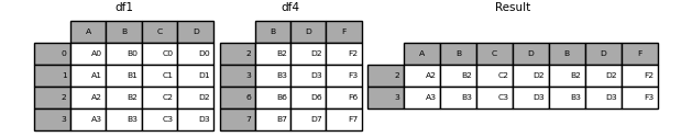
In [10]: result = pd.concat([df1, df4], axis=1, join='inner')

　　

 

Lastly, suppose we just wanted to reuse the exact index from the original DataFrame:

In [11]: result = pd.concat([df1, df4], axis=1, join_axes=[df1.index])

　　

 

Concatenating using append

A useful shortcut to concat are the append instance methods on Series and DataFrame. These methods actually predated concat. They concatenate along axis=0, namely the index:

In [12]: result = df1.append(df2)

　　

 

In the case of DataFrame, the indexes must be disjoint but the columns do not need to be:

In [13]: result = df1.append(df4)

　　

 

append may take multiple objects to concatenate:

In [14]: result = df1.append([df2, df3])

　　

 

Note

Unlike list.append method, which appends to the original list and returns nothing,append here does not modify df1 and returns its copy with df2 appended.

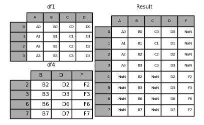
Ignoring indexes on the concatenation axis

For DataFrames which don’t have a meaningful index, you may wish to append them and ignore the fact that they may have overlapping indexes:

To do this, use the ignore_index argument:

In [15]: result = pd.concat([df1, df4], ignore_index=True)

　　

 

This is also a valid argument to DataFrame.append:

In [16]: result = df1.append(df4, ignore_index=True)

　　

 

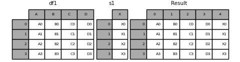
Concatenating with mixed ndims

You can concatenate a mix of Series and DataFrames. The Series will be transformed to DataFrames with the column name as the name of the Series.

In [17]: s1 = pd.Series(['X0', 'X1', 'X2', 'X3'], name='X')

In [18]: result = pd.concat([df1, s1], axis=1)

　　

 

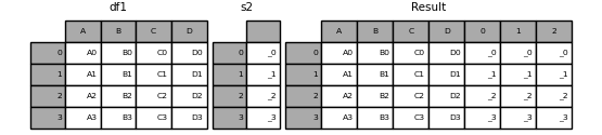
If unnamed Series are passed they will be numbered consecutively.

In [19]: s2 = pd.Series(['_0', '_1', '_2', '_3'])

In [20]: result = pd.concat([df1, s2, s2, s2], axis=1)

　　

 

Passing ignore_index=True will drop all name references.

In [21]: result = pd.concat([df1, s1], axis=1, ignore_index=True)

　　

 

More concatenating with group keys

A fairly common use of the keys argument is to override the column names when creating a new DataFrame based on existing Series. Notice how the default behaviour consists on letting the resulting DataFrame inherits the parent Series’ name, when these existed.

In [22]: s3 = pd.Series([0, 1, 2, 3], name='foo')

In [23]: s4 = pd.Series([0, 1, 2, 3])

In [24]: s5 = pd.Series([0, 1, 4, 5])

In [25]: pd.concat([s3, s4, s5], axis=1)
Out[25]:
   foo  0  1
0    0  0  0
1    1  1  1
2    2  2  4
3    3  3  5

　　

Through the keys argument we can override the existing column names.

In [26]: pd.concat([s3, s4, s5], axis=1, keys=['red','blue','yellow'])
Out[26]:
   red  blue  yellow
0    0     0       0
1    1     1       1
2    2     2       4
3    3     3       5

　　

Let’s consider now a variation on the very first example presented:

In [27]: result = pd.concat(frames, keys=['x', 'y', 'z'])

　　

 

You can also pass a dict to concat in which case the dict keys will be used for the keys argument (unless other keys are specified):

In [28]: pieces = {'x': df1, 'y': df2, 'z': df3}

In [29]: result = pd.concat(pieces)

　　

 

In [30]: result = pd.concat(pieces, keys=['z', 'y'])

　　

 

The MultiIndex created has levels that are constructed from the passed keys and the index of the DataFrame pieces:

In [31]: result.index.levels
Out[31]: FrozenList([[u'z', u'y'], [4, 5, 6, 7, 8, 9, 10, 11]])

　　

If you wish to specify other levels (as will occasionally be the case), you can do so using the levels argument:

In [32]: result = pd.concat(pieces, keys=['x', 'y', 'z'],
   ....:                 levels=[['z', 'y', 'x', 'w']],
   ....:                 names=['group_key'])
   ....:

　　

 

In [33]: result.index.levels
Out[33]: FrozenList([[u'z', u'y', u'x', u'w'], [0, 1, 2, 3, 4, 5, 6, 7, 8, 9, 10, 11]])

　　

Yes, this is fairly esoteric, but is actually necessary for implementing things like GroupBy where the order of a categorical variable is meaningful.

Appending rows to a DataFrame

While not especially efficient (since a new object must be created), you can append a single row to a DataFrame by passing a Series or dict to append, which returns a new DataFrame as above.

In [34]: s2 = pd.Series(['X0', 'X1', 'X2', 'X3'], index=['A', 'B', 'C', 'D'])

In [35]: result = df1.append(s2, ignore_index=True)

　　

 

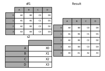
You should use ignore_index with this method to instruct DataFrame to discard its index. If you wish to preserve the index, you should construct an appropriately-indexed DataFrame and append or concatenate those objects.

You can also pass a list of dicts or Series:

In [36]: dicts = [{'A': 1, 'B': 2, 'C': 3, 'X': 4},
   ....:          {'A': 5, 'B': 6, 'C': 7, 'Y': 8}]
   ....: 

In [37]: result = df1.append(dicts, ignore_index=True)

　　

 

Database-style DataFrame joining/merging

pandas has full-featured, high performance in-memory join operations idiomatically very similar to relational databases like SQL. These methods perform significantly better (in some cases well over an order of magnitude better) than other open source implementations (like base::merge.data.frame in R). The reason for this is careful algorithmic design and internal layout of the data in DataFrame.

See the cookbook for some advanced strategies.

Users who are familiar with SQL but new to pandas might be interested in a comparison with SQL.

pandas provides a single function, merge, as the entry point for all standard database join operations between DataFrame objects:

pd.merge(left, right, how='inner', on=None, left_on=None, right_on=None,
         left_index=False, right_index=False, sort=True,
         suffixes=('_x', '_y'), copy=True, indicator=False)

　　

• left: A DataFrame object

• right: Another DataFrame object

• on: Columns (names) to join on. Must be found in both the left and right DataFrame objects. If not passed and left_index and right_index are False, the intersection of the columns in the DataFrames will be inferred to be the join keys

• left_on: Columns from the left DataFrame to use as keys. Can either be column names or arrays with length equal to the length of the DataFrame

• right_on: Columns from the right DataFrame to use as keys. Can either be column names or arrays with length equal to the length of the DataFrame

• left_index: If True, use the index (row labels) from the left DataFrame as its join key(s). In the case of a DataFrame with a MultiIndex (hierarchical), the number of levels must match the number of join keys from the right DataFrame

• right_index: Same usage as left_index for the right DataFrame

• how: One of 'left', 'right', 'outer', 'inner'. Defaults to inner. See below for more detailed description of each method

• sort: Sort the result DataFrame by the join keys in lexicographical order. Defaults to True, setting to False will improve performance substantially in many cases

• suffixes: A tuple of string suffixes to apply to overlapping columns. Defaults to ('_x', '_y').

• copy: Always copy data (default True) from the passed DataFrame objects, even when reindexing is not necessary. Cannot be avoided in many cases but may improve performance / memory usage. The cases where copying can be avoided are somewhat pathological but this option is provided nonetheless.

• indicator: Add a column to the output DataFrame called _merge with information on the source of each row. _merge is Categorical-type and takes on a value of left_only for observations whose merge key only appears in 'left' DataFrame, right_only for observations whose merge key only appears in 'right' DataFrame, and both if the observation’s merge key is found in both.

  New in version 0.17.0.

The return type will be the same as left. If left is a DataFrame and right is a subclass of DataFrame, the return type will still be DataFrame.

merge is a function in the pandas namespace, and it is also available as a DataFrame instance method, with the calling DataFrame being implicitly considered the left object in the join.

The related DataFrame.join method, uses merge internally for the index-on-index (by default) and column(s)-on-index join. If you are joining on index only, you may wish to use DataFrame.join to save yourself some typing.

Brief primer on merge methods (relational algebra)

Experienced users of relational databases like SQL will be familiar with the terminology used to describe join operations between two SQL-table like structures (DataFrame objects). There are several cases to consider which are very important to understand:

• one-to-one joins: for example when joining two DataFrame objects on their indexes (which must contain unique values)
• many-to-one joins: for example when joining an index (unique) to one or more columns in a DataFrame
• many-to-many joins: joining columns on columns.

Note

When joining columns on columns (potentially a many-to-many join), any indexes on the passed DataFrame objects will be discarded.

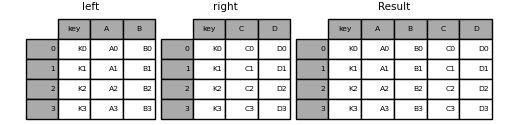
It is worth spending some time understanding the result of the many-to-many join case. In SQL / standard relational algebra, if a key combination appears more than once in both tables, the resulting table will have the Cartesian product of the associated data. Here is a very basic example with one unique key combination:

In [38]: left = pd.DataFrame({'key': ['K0', 'K1', 'K2', 'K3'],
   ....:                      'A': ['A0', 'A1', 'A2', 'A3'],
   ....:                      'B': ['B0', 'B1', 'B2', 'B3']})
   ....: 

In [39]: right = pd.DataFrame({'key': ['K0', 'K1', 'K2', 'K3'],
   ....:                       'C': ['C0', 'C1', 'C2', 'C3'],
   ....:                       'D': ['D0', 'D1', 'D2', 'D3']})
   ....: 

In [40]: result = pd.merge(left, right, on='key')

　　

 

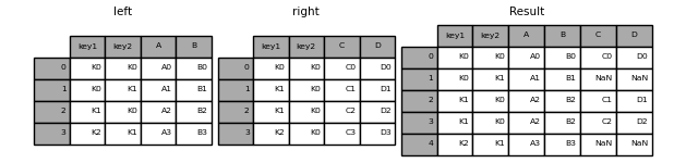
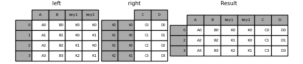
Here is a more complicated example with multiple join keys:

In [41]: left = pd.DataFrame({'key1': ['K0', 'K0', 'K1', 'K2'],
   ....:                      'key2': ['K0', 'K1', 'K0', 'K1'],
   ....:                      'A': ['A0', 'A1', 'A2', 'A3'],
   ....:                      'B': ['B0', 'B1', 'B2', 'B3']})
   ....: 

In [42]: right = pd.DataFrame({'key1': ['K0', 'K1', 'K1', 'K2'],
   ....:                       'key2': ['K0', 'K0', 'K0', 'K0'],
   ....:                       'C': ['C0', 'C1', 'C2', 'C3'],
   ....:                       'D': ['D0', 'D1', 'D2', 'D3']})
   ....: 

In [43]: result = pd.merge(left, right, on=['key1', 'key2'])

　　

 

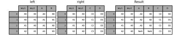
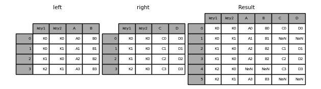
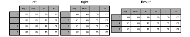
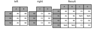
The how argument to merge specifies how to determine which keys are to be included in the resulting table. If a key combination does not appear in either the left or right tables, the values in the joined table will be NA. Here is a summary of the how options and their SQL equivalent names:

Merge method	SQL Join Name	Description
left	LEFT OUTER JOIN	Use keys from left frame only
right	RIGHT OUTER JOIN	Use keys from right frame only
outer	FULL OUTER JOIN	Use union of keys from both frames
inner	INNER JOIN	Use intersection of keys from both frames

In [44]: result = pd.merge(left, right, how='left', on=['key1', 'key2'])

　　

 

In [45]: result = pd.merge(left, right, how='right', on=['key1', 'key2'])

　　

 

In [46]: result = pd.merge(left, right, how='outer', on=['key1', 'key2'])

　　

 

In [47]: result = pd.merge(left, right, how='inner', on=['key1', 'key2'])

　　

 

The merge indicator

New in version 0.17.0.

merge now accepts the argument indicator. If True, a Categorical-type column called _merge will be added to the output object that takes on values:

Observation Origin	_merge value
Merge key only in 'left' frame	left_only
Merge key only in 'right' frame	right_only
Merge key in both frames	both

In [48]: df1 = pd.DataFrame({'col1': [0, 1], 'col_left':['a', 'b']})

In [49]: df2 = pd.DataFrame({'col1': [1, 2, 2],'col_right':[2, 2, 2]})

In [50]: pd.merge(df1, df2, on='col1', how='outer', indicator=True)
Out[50]:
   col1 col_left  col_right      _merge
0     0        a        NaN   left_only
1     1        b        2.0        both
2     2      NaN        2.0  right_only
3     2      NaN        2.0  right_only

　　

The indicator argument will also accept string arguments, in which case the indicator function will use the value of the passed string as the name for the indicator column.

In [51]: pd.merge(df1, df2, on='col1', how='outer', indicator='indicator_column')
Out[51]:
   col1 col_left  col_right indicator_column
0     0        a        NaN        left_only
1     1        b        2.0             both
2     2      NaN        2.0       right_only
3     2      NaN        2.0       right_only

　　

Joining on index

DataFrame.join is a convenient method for combining the columns of two potentially differently-indexed DataFrames into a single result DataFrame. Here is a very basic example:

In [52]: left = pd.DataFrame({'A': ['A0', 'A1', 'A2'],
   ....:                      'B': ['B0', 'B1', 'B2']},
   ....:                      index=['K0', 'K1', 'K2'])
   ....: 

In [53]: right = pd.DataFrame({'C': ['C0', 'C2', 'C3'],
   ....:                       'D': ['D0', 'D2', 'D3']},
   ....:                       index=['K0', 'K2', 'K3'])
   ....: 

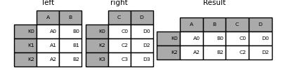
In [54]: result = left.join(right)

　　

 

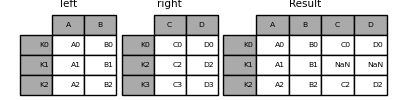
In [55]: result = left.join(right, how='outer')

　　

 

In [56]: result = left.join(right, how='inner')

　　

 

The data alignment here is on the indexes (row labels). This same behavior can be achieved using merge plus additional arguments instructing it to use the indexes:

In [57]: result = pd.merge(left, right, left_index=True, right_index=True, how='outer')

　　

 

In [58]: result = pd.merge(left, right, left_index=True, right_index=True, how='inner');

　　

 

Joining key columns on an index

join takes an optional on argument which may be a column or multiple column names, which specifies that the passed DataFrame is to be aligned on that column in the DataFrame. These two function calls are completely equivalent:

left.join(right, on=key_or_keys)
pd.merge(left, right, left_on=key_or_keys, right_index=True,
      how='left', sort=False)

　　

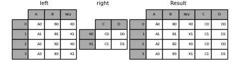
Obviously you can choose whichever form you find more convenient. For many-to-one joins (where one of the DataFrame’s is already indexed by the join key), using join may be more convenient. Here is a simple example:

In [59]: left = pd.DataFrame({'A': ['A0', 'A1', 'A2', 'A3'],
   ....:                      'B': ['B0', 'B1', 'B2', 'B3'],
   ....:                      'key': ['K0', 'K1', 'K0', 'K1']})
   ....: 

In [60]: right = pd.DataFrame({'C': ['C0', 'C1'],
   ....:                       'D': ['D0', 'D1']},
   ....:                       index=['K0', 'K1'])
   ....: 

In [61]: result = left.join(right, on='key')

　　

 

In [62]: result = pd.merge(left, right, left_on='key', right_index=True,
   ....:                   how='left', sort=False);
   ....:

　　

 

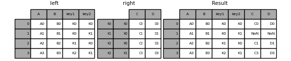
To join on multiple keys, the passed DataFrame must have a MultiIndex:

In [63]: left = pd.DataFrame({'A': ['A0', 'A1', 'A2', 'A3'],
   ....:                      'B': ['B0', 'B1', 'B2', 'B3'],
   ....:                      'key1': ['K0', 'K0', 'K1', 'K2'],
   ....:                      'key2': ['K0', 'K1', 'K0', 'K1']})
   ....: 

In [64]: index = pd.MultiIndex.from_tuples([('K0', 'K0'), ('K1', 'K0'),
   ....:                                   ('K2', 'K0'), ('K2', 'K1')])
   ....: 

In [65]: right = pd.DataFrame({'C': ['C0', 'C1', 'C2', 'C3'],
   ....:                    'D': ['D0', 'D1', 'D2', 'D3']},
   ....:                   index=index)
   ....:

　　

Now this can be joined by passing the two key column names:

In [66]: result = left.join(right, on=['key1', 'key2'])

　　

 

The default for DataFrame.join is to perform a left join (essentially a “VLOOKUP” operation, for Excel users), which uses only the keys found in the calling DataFrame. Other join types, for example inner join, can be just as easily performed:

In [67]: result = left.join(right, on=['key1', 'key2'], how='inner')

　　

 

As you can see, this drops any rows where there was no match.

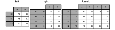
Joining a single Index to a Multi-index

New in version 0.14.0.

You can join a singly-indexed DataFrame with a level of a multi-indexed DataFrame. The level will match on the name of the index of the singly-indexed frame against a level name of the multi-indexed frame.

In [68]: left = pd.DataFrame({'A': ['A0', 'A1', 'A2'],
   ....:                      'B': ['B0', 'B1', 'B2']},
   ....:                      index=pd.Index(['K0', 'K1', 'K2'], name='key'))
   ....: 

In [69]: index = pd.MultiIndex.from_tuples([('K0', 'Y0'), ('K1', 'Y1'),
   ....:                                   ('K2', 'Y2'), ('K2', 'Y3')],
   ....:                                    names=['key', 'Y'])
   ....: 

In [70]: right = pd.DataFrame({'C': ['C0', 'C1', 'C2', 'C3'],
   ....:                       'D': ['D0', 'D1', 'D2', 'D3']},
   ....:                       index=index)
   ....: 

In [71]: result = left.join(right, how='inner')

　　

 

This is equivalent but less verbose and more memory efficient / faster than this.

In [72]: result = pd.merge(left.reset_index(), right.reset_index(),
   ....:       on=['key'], how='inner').set_index(['key','Y'])
   ....:

　　

 

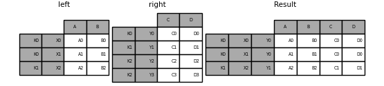
Joining with two multi-indexes

This is not Implemented via join at-the-moment, however it can be done using the following.

In [73]: index = pd.MultiIndex.from_tuples([('K0', 'X0'), ('K0', 'X1'),
   ....:                                    ('K1', 'X2')],
   ....:                                     names=['key', 'X'])
   ....: 

In [74]: left = pd.DataFrame({'A': ['A0', 'A1', 'A2'],
   ....:                      'B': ['B0', 'B1', 'B2']},
   ....:                       index=index)
   ....: 

In [75]: result = pd.merge(left.reset_index(), right.reset_index(),
   ....:                   on=['key'], how='inner').set_index(['key','X','Y'])
   ....:

　　

 

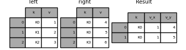
Overlapping value columns

The merge suffixes argument takes a tuple of list of strings to append to overlapping column names in the input DataFrames to disambiguate the result columns:

In [76]: left = pd.DataFrame({'k': ['K0', 'K1', 'K2'], 'v': [1, 2, 3]})

In [77]: right = pd.DataFrame({'k': ['K0', 'K0', 'K3'], 'v': [4, 5, 6]})

In [78]: result = pd.merge(left, right, on='k')

　　

 

In [79]: result = pd.merge(left, right, on='k', suffixes=['_l', '_r'])

　　

 

DataFrame.join has lsuffix and rsuffix arguments which behave similarly.

In [80]: left = left.set_index('k')

In [81]: right = right.set_index('k')

In [82]: result = left.join(right, lsuffix='_l', rsuffix='_r')

　　

 

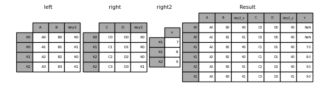
Joining multiple DataFrame or Panel objects

A list or tuple of DataFrames can also be passed to DataFrame.join to join them together on their indexes. The same is true for Panel.join.

In [83]: right2 = pd.DataFrame({'v': [7, 8, 9]}, index=['K1', 'K1', 'K2'])

In [84]: result = left.join([right, right2])

　　

 

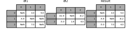
Merging together values within Series or DataFrame columns

Another fairly common situation is to have two like-indexed (or similarly indexed) Series or DataFrame objects and wanting to “patch” values in one object from values for matching indices in the other. Here is an example:

In [85]: df1 = pd.DataFrame([[np.nan, 3., 5.], [-4.6, np.nan, np.nan],
   ....:                    [np.nan, 7., np.nan]])
   ....: 

In [86]: df2 = pd.DataFrame([[-42.6, np.nan, -8.2], [-5., 1.6, 4]],
   ....:                    index=[1, 2])
   ....:

　　

For this, use the combine_first method:

In [87]: result = df1.combine_first(df2)

　　

 

Note that this method only takes values from the right DataFrame if they are missing in the left DataFrame. A related method, update, alters non-NA values inplace:

In [88]: df1.update(df2)

　　

 

Timeseries friendly merging

Merging Ordered Data

A merge_ordered() function allows combining time series and other ordered data. In particular it has an optional fill_method keyword to fill/interpolate missing data:

In [89]: left = pd.DataFrame({'k': ['K0', 'K1', 'K1', 'K2'],
   ....:                      'lv': [1, 2, 3, 4],
   ....:                      's': ['a', 'b', 'c', 'd']})
   ....: 

In [90]: right = pd.DataFrame({'k': ['K1', 'K2', 'K4'],
   ....:                       'rv': [1, 2, 3]})
   ....: 

In [91]: pd.merge_ordered(left, right, fill_method='ffill', left_by='s')
Out[91]:
     k   lv  s   rv
0   K0  1.0  a  NaN
1   K1  1.0  a  1.0
2   K2  1.0  a  2.0
3   K4  1.0  a  3.0
4   K1  2.0  b  1.0
5   K2  2.0  b  2.0
6   K4  2.0  b  3.0
7   K1  3.0  c  1.0
8   K2  3.0  c  2.0
9   K4  3.0  c  3.0
10  K1  NaN  d  1.0
11  K2  4.0  d  2.0
12  K4  4.0  d  3.0

　　

Merging AsOf

New in version 0.19.0.

A merge_asof() is similar to an ordered left-join except that we match on nearest key rather than equal keys. For each row in the left DataFrame, we select the last row in the right DataFrame whose on key is less than the left’s key. Both DataFrames must be sorted by the key.

Optionally an asof merge can perform a group-wise merge. This matches the by key equally, in addition to the nearest match on the on key.

For example; we might have trades and quotes and we want to asof merge them.

In [92]: trades = pd.DataFrame({
   ....:     'time': pd.to_datetime(['20160525 13:30:00.023',
   ....:                             '20160525 13:30:00.038',
   ....:                             '20160525 13:30:00.048',
   ....:                             '20160525 13:30:00.048',
   ....:                             '20160525 13:30:00.048']),
   ....:     'ticker': ['MSFT', 'MSFT',
   ....:                'GOOG', 'GOOG', 'AAPL'],
   ....:     'price': [51.95, 51.95,
   ....:               720.77, 720.92, 98.00],
   ....:     'quantity': [75, 155,
   ....:                  100, 100, 100]},
   ....:     columns=['time', 'ticker', 'price', 'quantity'])
   ....: 

In [93]: quotes = pd.DataFrame({
   ....:     'time': pd.to_datetime(['20160525 13:30:00.023',
   ....:                             '20160525 13:30:00.023',
   ....:                             '20160525 13:30:00.030',
   ....:                             '20160525 13:30:00.041',
   ....:                             '20160525 13:30:00.048',
   ....:                             '20160525 13:30:00.049',
   ....:                             '20160525 13:30:00.072',
   ....:                             '20160525 13:30:00.075']),
   ....:     'ticker': ['GOOG', 'MSFT', 'MSFT',
   ....:                'MSFT', 'GOOG', 'AAPL', 'GOOG',
   ....:                'MSFT'],
   ....:     'bid': [720.50, 51.95, 51.97, 51.99,
   ....:             720.50, 97.99, 720.50, 52.01],
   ....:     'ask': [720.93, 51.96, 51.98, 52.00,
   ....:             720.93, 98.01, 720.88, 52.03]},
   ....:     columns=['time', 'ticker', 'bid', 'ask'])
   ....:

　　

In [94]: trades
Out[94]:
                     time ticker   price  quantity
0 2016-05-25 13:30:00.023   MSFT   51.95        75
1 2016-05-25 13:30:00.038   MSFT   51.95       155
2 2016-05-25 13:30:00.048   GOOG  720.77       100
3 2016-05-25 13:30:00.048   GOOG  720.92       100
4 2016-05-25 13:30:00.048   AAPL   98.00       100

In [95]: quotes
Out[95]:
                     time ticker     bid     ask
0 2016-05-25 13:30:00.023   GOOG  720.50  720.93
1 2016-05-25 13:30:00.023   MSFT   51.95   51.96
2 2016-05-25 13:30:00.030   MSFT   51.97   51.98
3 2016-05-25 13:30:00.041   MSFT   51.99   52.00
4 2016-05-25 13:30:00.048   GOOG  720.50  720.93
5 2016-05-25 13:30:00.049   AAPL   97.99   98.01
6 2016-05-25 13:30:00.072   GOOG  720.50  720.88
7 2016-05-25 13:30:00.075   MSFT   52.01   52.03

　　

By default we are taking the asof of the quotes.

In [96]: pd.merge_asof(trades, quotes,
   ....:               on='time',
   ....:               by='ticker')
   ....:
Out[96]:
                     time ticker   price  quantity     bid     ask
0 2016-05-25 13:30:00.023   MSFT   51.95        75   51.95   51.96
1 2016-05-25 13:30:00.038   MSFT   51.95       155   51.97   51.98
2 2016-05-25 13:30:00.048   GOOG  720.77       100  720.50  720.93
3 2016-05-25 13:30:00.048   GOOG  720.92       100  720.50  720.93
4 2016-05-25 13:30:00.048   AAPL   98.00       100     NaN     NaN

　　

We only asof within 2ms betwen the quote time and the trade time.

In [97]: pd.merge_asof(trades, quotes,
   ....:               on='time',
   ....:               by='ticker',
   ....:               tolerance=pd.Timedelta('2ms'))
   ....:
Out[97]:
                     time ticker   price  quantity     bid     ask
0 2016-05-25 13:30:00.023   MSFT   51.95        75   51.95   51.96
1 2016-05-25 13:30:00.038   MSFT   51.95       155     NaN     NaN
2 2016-05-25 13:30:00.048   GOOG  720.77       100  720.50  720.93
3 2016-05-25 13:30:00.048   GOOG  720.92       100  720.50  720.93
4 2016-05-25 13:30:00.048   AAPL   98.00       100     NaN     NaN

　　

We only asof within 10ms betwen the quote time and the trade time and we exclude exact matches on time. Note that though we exclude the exact matches (of the quotes), prior quotes DO propogate to that point in time.

In [98]: pd.merge_asof(trades, quotes,
   ....:               on='time',
   ....:               by='ticker',
   ....:               tolerance=pd.Timedelta('10ms'),
   ....:               allow_exact_matches=False)
   ....:
Out[98]:
                     time ticker   price  quantity    bid    ask
0 2016-05-25 13:30:00.023   MSFT   51.95        75    NaN    NaN
1 2016-05-25 13:30:00.038   MSFT   51.95       155  51.97  51.98
2 2016-05-25 13:30:00.048   GOOG  720.77       100    NaN    NaN
3 2016-05-25 13:30:00.048   GOOG  720.92       100    NaN    NaN
4 2016-05-25 13:30:00.048   AAPL   98.00       100    NaN    NaN