TensorFlow使用记录 (七）： BN 层及 Dropout 层的使用

参考：tensorflow中的batch_norm以及tf.control_dependencies和tf.GraphKeys.UPDATE_OPS的探究

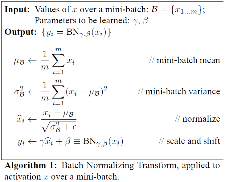
1. Batch Normalization

对卷积层来说，批量归一化发生在卷积计算之后、应用激活函数之前。训练阶段：如果卷积计算输出多个通道，我们需要对这些通道的输出分别做批量归一化，且每个通道都拥有独立的拉伸和偏移参数，并均为标量。假设小批量中有 m 个样本。在单个通道上，假设卷积计算输出的高和宽分别为p和q。我们需要对该通道中m×p×q个元素同时做批量归一化。对这些元素做标准化计算时，我们使用相同的均值和方差，即该通道中m×p×q个元素的均值和方差。测试阶段：就直接用训练阶段利用 moving average 方式获得的整个训练集的 均值和方差来归一化。

以一个 mxnet 版本的代码来理解具体实现吧：

def batch_norm(X, gamma, beta, moving_mean, moving_var, eps, momentum):
    # 通过autograd来判断当前模式是训练模式还是预测模式
    if not autograd.is_training():
        # 如果是在预测模式下，直接使用传入的移动平均所得的均值和方差
        X_hat = (X - moving_mean) / nd.sqrt(moving_var + eps)
    else:
        assert len(X.shape) in (2, 4)
        if len(X.shape) == 2:
            # 使用全连接层的情况，计算特征维上的均值和方差
            mean = X.mean(axis=0)
            var = ((X - mean) ** 2).mean(axis=0)
        else:
            # 使用二维卷积层的情况，计算通道维上（axis=1）的均值和方差。这里我们需要保持
            # X的形状以便后面可以做广播运算
            mean = X.mean(axis=(0, 2, 3), keepdims=True)
            var = ((X - mean) ** 2).mean(axis=(0, 2, 3), keepdims=True)
        # 训练模式下用当前的均值和方差做标准化
        X_hat = (X - mean) / nd.sqrt(var + eps)
        # 更新移动平均的均值和方差
        moving_mean = momentum * moving_mean + (1.0 - momentum) * mean
        moving_var = momentum * moving_var + (1.0 - momentum) * var
    Y = gamma * X_hat + beta  # 拉伸和偏移
    return Y, moving_mean, moving_var

class BatchNorm(nn.Block):
    def __init__(self, num_features, num_dims, **kwargs):
        super(BatchNorm, self).__init__(**kwargs)
        if num_dims == 2:
            shape = (1, num_features)
        else:
            shape = (1, num_features, 1, 1)
        # 参与求梯度和迭代的拉伸和偏移参数，分别初始化成1和0
        self.gamma = self.params.get('gamma', shape=shape, init=init.One())
        self.beta = self.params.get('beta', shape=shape, init=init.Zero())
        # 不参与求梯度和迭代的变量，全在内存上初始化成0
        self.moving_mean = nd.zeros(shape)
        self.moving_var = nd.zeros(shape)

    def forward(self, X):
        # 如果X不在内存上，将moving_mean和moving_var复制到X所在显存上
        if self.moving_mean.context != X.context:
            self.moving_mean = self.moving_mean.copyto(X.context)
            self.moving_var = self.moving_var.copyto(X.context)
        # 保存更新过的moving_mean和moving_var
        Y, self.moving_mean, self.moving_var = batch_norm(
            X, self.gamma.data(), self.beta.data(), self.moving_mean,
            self.moving_var, eps=1e-5, momentum=0.9)
        return Y

2. TensorFlow 实现

tensorflow中关于batch_norm现在有三种实现方式。

2.1 tf.nn.batch_normalization

tf.nn.batch_normalization(
    x,
    mean,
    variance,
    offset,
    scale,
    variance_epsilon,
    name=None
)

该函数是一种最底层的实现方法，在使用时mean、variance、scale、offset等参数需要自己传递并更新，因此实际使用时还需自己对该函数进行封装，一般不建议使用，但是对了解batch_norm的原理很有帮助。

import tensorflow as tf

def batch_norm(x, name_scope, training, epsilon=1e-3, decay=0.99):
    """ Assume nd [batch, N1, N2, ..., Nm, Channel] tensor"""
    with tf.variable_scope(name_scope):
        size = x.get_shape().as_list()[-1]
        scale = tf.get_variable('scale', [size], initializer=tf.constant_initializer(0.1))
        offset = tf.get_variable('offset', [size])

        pop_mean = tf.get_variable('pop_mean', [size], initializer=tf.zeros_initializer(), trainable=False)
        pop_var = tf.get_variable('pop_var', [size], initializer=tf.ones_initializer(), trainable=False)
        batch_mean, batch_var = tf.nn.moments(x, list(range(len(x.get_shape())-1)))
        train_mean_op = tf.assign(pop_mean, pop_mean * decay + batch_mean * (1 - decay))
        train_var_op = tf.assign(pop_var, pop_var * decay + batch_var * (1 - decay))

        def batch_statistics():
            with tf.control_dependencies([train_mean_op, train_var_op]):
                return tf.nn.batch_normalization(x, batch_mean, batch_var, offset, scale, epsilon)
        def population_statistics():
            return tf.nn.batch_normalization(x, pop_mean, pop_var, offset, scale, epsilon)

        return tf.cond(training, batch_statistics, population_statistics)

is_traing = tf.placeholder(dtype=tf.bool)
input = tf.ones([1, 2, 2, 3])
output = batch_norm(input, name_scope='batch_norm_nn', training=is_traing)

2.2 tf.layers.batch_normalization

tf.layers.batch_normalization(
    inputs,
    axis=-1,
    momentum=0.99,
    epsilon=0.001,
    center=True,
    scale=True,
    beta_initializer=tf.zeros_initializer(),
    gamma_initializer=tf.ones_initializer(),
    moving_mean_initializer=tf.zeros_initializer(),
    moving_variance_initializer=tf.ones_initializer(),
    beta_regularizer=None,
    gamma_regularizer=None,
    beta_constraint=None,
    gamma_constraint=None,
    training=False,
    trainable=True,
    name=None,
    reuse=None,
    renorm=False,
    renorm_clipping=None,
    renorm_momentum=0.99,
    fused=None,
    virtual_batch_size=None,
    adjustment=None
)
"""
Note: when training, the moving_mean and moving_variance need to be updated.
By default the update ops are placed in `tf.GraphKeys.UPDATE_OPS`, so they
need to be executed alongside the `train_op`. Also, be sure to add any
batch_normalization ops before getting the update_ops collection. Otherwise,
update_ops will be empty, and training/inference will not work properly. For
example:

```python
x_norm = tf.compat.v1.layers.batch_normalization(x, training=training)

# ...

update_ops = tf.compat.v1.get_collection(tf.GraphKeys.UPDATE_OPS)
train_op = optimizer.minimize(loss)
train_op = tf.group([train_op, update_ops])
```
"""

以下是个完整的 MNIST 训练网络：

import tensorflow as tf

# 1. create data
from tensorflow.examples.tutorials.mnist import input_data
mnist = input_data.read_data_sets('../MNIST_data', one_hot=True)

X = tf.placeholder(tf.float32, shape=(None, 784), name='X')
y = tf.placeholder(tf.int32, shape=(None), name='y')
is_training = tf.placeholder(tf.bool, None, name='is_training')

# 2. define network
he_init = tf.initializers.he_normal()
xavier_init = tf.initializers.glorot_normal()
with tf.name_scope('dnn'):
    hidden1 = tf.layers.dense(X, 300, kernel_initializer=he_init, name='hidden1')
    hidden1 = tf.layers.batch_normalization(hidden1, momentum=0.9)
    hidden1 = tf.nn.relu(hidden1)
    hidden2 = tf.layers.dense(hidden1, 100, kernel_initializer=he_init, name='hidden2')
    hidden2 = tf.layers.batch_normalization(hidden2, training=is_training, momentum=0.9)
    hidden2 = tf.nn.relu(hidden2)
    logits = tf.layers.dense(hidden2, 10, kernel_initializer=he_init, name='output')
    # prob = tf.layers.dense(hidden2, 10, tf.nn.softmax, name='prob')

# 3. define loss
with tf.name_scope('loss'):
    # tf.losses.sparse_softmax_cross_entropy() label is not one_hot and dtype is int*
    # xentropy = tf.losses.sparse_softmax_cross_entropy(labels=tf.argmax(y, axis=1), logits=logits)
    # tf.nn.sparse_softmax_cross_entropy_with_logits() label is not one_hot and dtype is int*
    # xentropy = tf.nn.sparse_softmax_cross_entropy_with_logits(labels=tf.argmax(y, axis=1), logits=logits)
    # loss = tf.reduce_mean(xentropy)
    loss = tf.losses.softmax_cross_entropy(onehot_labels=y, logits=logits) # label is one_hot

# 4. define optimizer
learning_rate = 0.01
with tf.name_scope('train'):
    update_ops = tf.get_collection(tf.GraphKeys.UPDATE_OPS)  # for batch normalization
    with tf.control_dependencies(update_ops):
        optimizer_op = tf.train.GradientDescentOptimizer(learning_rate).minimize(loss)

with tf.name_scope('eval'):
    correct = tf.nn.in_top_k(logits, tf.argmax(y, axis=1), 1) # 目标是否在前K个预测中, label's dtype is int*
    accuracy = tf.reduce_mean(tf.cast(correct, tf.float32))

# 5. initialize
init_op = tf.group(tf.global_variables_initializer(), tf.local_variables_initializer())
saver = tf.train.Saver()
# =================
print([v.name for v in tf.trainable_variables()])
print([v.name for v in tf.global_variables()])
# =================
# 5. train & test
n_epochs = 20
n_batches = 50
batch_size = 50

with tf.Session() as sess:
    sess.run(init_op)
    for epoch in range(n_epochs):
        for iteration in range(mnist.train.num_examples // batch_size):
            X_batch, y_batch = mnist.train.next_batch(batch_size)
            sess.run(optimizer_op, feed_dict={X: X_batch, y: y_batch, is_training:True})
        acc_train = accuracy.eval(feed_dict={X: X_batch, y: y_batch, is_training:False}) # 最后一个 batch 的 accuracy
        acc_test = accuracy.eval(feed_dict={X: mnist.test.images, y: mnist.test.labels, is_training:False})
        loss_test = loss.eval(feed_dict={X: mnist.test.images, y: mnist.test.labels, is_training:False})
        print(epoch, "Train accuracy:", acc_train, "Test accuracy:", acc_test, "Test loss:", loss_test)
    save_path = saver.save(sess, "./my_model_final.ckpt")

with tf.Session() as sess:
    sess.run(init_op)
    saver.restore(sess, "./my_model_final.ckpt")
    acc_test = accuracy.eval(feed_dict={X: mnist.test.images, y: mnist.test.labels, is_training:False})
    loss_test = loss.eval(feed_dict={X: mnist.test.images, y: mnist.test.labels, is_training:False})
    print("Test accuracy:", acc_test, ", Test loss:", loss_test)

2.3 tf.contrib.layers.batch_norm

涉及到 contribe 部分就先 pass 吧

3. 关于tf.GraphKeys.UPDATA_OPS

3.1 tf.control_dependencies

按照下面这个例子理解下：

import tensorflow as tf

a_1 = tf.Variable(1)
b_1 = tf.Variable(2)
update_op = tf.assign(a_1, 10)
add = tf.add(a_1, b_1)

a_2 = tf.Variable(1)
b_2 = tf.Variable(2)
update_op2 = tf.assign(a_2, 10)
with tf.control_dependencies([update_op2]):
    add_with_dependencies = tf.add(a_2, b_2)

init = tf.group(tf.global_variables_initializer(), tf.local_variables_initializer())
with tf.Session() as sess:
    sess.run(init)
    ans_1, ans_2 = sess.run([add, add_with_dependencies])
    print("Add: ", ans_1)
    print("Add_with_dependency: ", ans_2)

"""
可以看到两组加法进行的对比，正常的计算图在计算 add 时是不会经过 update_op 操作的，
因此在加法时 a 的值仍为 1，但是采用 tf.control_dependencies 函数，可以控制在进行
add 前先完成 update_op 的操作，因此在加法时 a 的值为 10，因此最后两种加法的结果不同。
"""

3.2 tf.GraphKeys.UPDATE_OPS

关于 tf.GraphKeys.UPDATE_OPS，这是一个 tensorflow 的计算图中内置的一个集合，其中会保存一些需要在训练操作之前完成的操作，并配合 tf.control_dependencies 函数使用。
关于在 batch_norm 中，即为更新 mean 和 variance 的操作。通过下面一个例子可以看到 tf.layers.batch_normalization 中是如何实现的。

import tensorflow as tf

is_traing = tf.placeholder(dtype=tf.bool, shape=None)
input = tf.ones([1, 2, 2, 3])
output = tf.layers.batch_normalization(input, training=is_traing)

update_ops = tf.get_collection(tf.GraphKeys.UPDATE_OPS)
print(update_ops)
print([v.name for v in tf.trainable_variables()])
print([v.name for v in tf.global_variables()])

"""
[<tf.Operation 'batch_normalization/AssignMovingAvg' type=AssignSub>, <tf.Operation 'batch_normalization/AssignMovingAvg_1' type=AssignSub>]
['batch_normalization/gamma:0', 'batch_normalization/beta:0']
['batch_normalization/gamma:0', 'batch_normalization/beta:0', 'batch_normalization/moving_mean:0', 'batch_normalization/moving_variance:0']
"""

可以看到输出的即为两个 batch_normalization 中更新 mean 和 variance 的操作，需要保证它们在 train_op 前完成。
这两个操作是在 tensorflow 的内部实现中自动被加入 tf.GraphKeys.UPDATE_OPS 这个集合的，在 tf.contrib.layers.batch_norm 的参数中可以看到有一项 updates_collections 的默认值即为 tf.GraphKeys.UPDATE_OPS，而在 tf.layers.batch_normalization 中则是直接将两个更新操作放入了上述集合。

如果在使用时不添加 tf.control_dependencies 函数，即在训练时(training=True)每批次时只会计算当批次的 mean 和 var，并传递给 tf.nn.batch_normalization 进行归一化，由于 mean_update 和 variance_update 在计算图中并不在上述操作的依赖路径上，因为并不会主动完成，也就是说，在训练时 mean_update 和 variance_update 并不会被使用到，其值一直是初始值。因此在测试阶段(training=False)使用这两个作为 mean 和 variance 并进行归一化操作，这样就会尴尬了。而如果使用 tf.control_dependencies 函数，会在训练阶段每次训练操作执行前被动地去执行 mean_update 和 variance_update，因此 moving_mean 和 moving_variance 会被不断更新，在测试时使用该参数也就不会有问题了。

One more thing: notice that the list of trainable variables is shorter than the list of all global variables. This is because the moving averages are non-trainable variables. If you want to reuse a pretrained neural network (see below), you must not forget these non-trainable variables.

4. Dropout

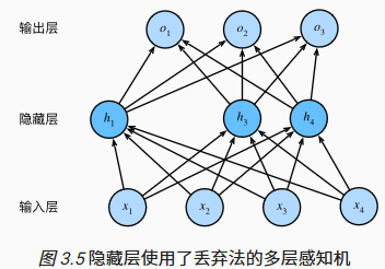
以上图为例，对隐含层做概率为 $p$ 的Dropout操作时，有 $p$ 的概率 $h_i$ 会被清零，而又 $1-p$ 的概率 $h_i$ 会除以 $1-p$ 做拉伸。目的是在不改变隐含层的期望值的前提下，用随机丢弃的方式使得输出层的计算无法过度依赖于隐含层的任节点。

def dropout(X, drop_prob):
    assert 0 <= drop_prob <= 1
    keep_prob = 1 - drop_prob
    # 这种情况下把全部元素都丢弃
    if keep_prob == 0:
        return X.zeros_like()
    mask = nd.random.uniform(0, 1, X.shape) < keep_prob
    return mask * X / keep_prob

tf.nn.dropout

tf.nn.dropout(
    x,
    keep_prob=None,
    noise_shape=None,
    seed=None,
    name=None,
    rate=None
)

以下是一个是否使用 Dropout 训练的实例：

import tensorflow as tf
import numpy as np
import matplotlib.pyplot as plt

print(tf.__version__)

# Hyper parameters
tf.set_random_seed(1)
np.random.seed(1)
N_SAMPLES = 20  # 样本点数
N_HIDDEN = 300  # 隐含层节点数
LR = 0.01  # 初始学习率

# 1. create data
x_train = np.linspace(-1, 1, N_SAMPLES)[:, np.newaxis]
y_train = x_train + 0.3 * np.random.randn(N_SAMPLES)[:, np.newaxis]

x_test = x_train.copy()
y_test = x_test + 0.3 * np.random.randn(N_SAMPLES)[:, np.newaxis]

# show data
plt.scatter(x_train, y_train, c='magenta', s=50, alpha=0.5, label='train')
plt.scatter(x_test, y_test, c='cyan', s=50, alpha=0.5, label='test')
plt.legend(loc='upper left')
plt.show()

# tf placeholder
tf_x = tf.placeholder(tf.float32, [None, 1])
tf_y = tf.placeholder(tf.float32, [None, 1])
is_training = tf.placeholder(tf.bool, None)  # to control dropout

# 2. construct network
o1 = tf.layers.dense(tf_x, N_HIDDEN, tf.nn.relu)
o2 = tf.layers.dense(o1, N_HIDDEN, tf.nn.relu)
o_predict = tf.layers.dense(o2, 1)
# ==========
d1 = tf.layers.dense(tf_x, N_HIDDEN, tf.nn.relu)
d1 = tf.layers.dropout(d1, rate=0.5, training=is_training)  # drop out 50%
d2 = tf.layers.dense(d1, N_HIDDEN, tf.nn.relu)
d2 = tf.layers.dropout(d2, rate=0.5, training=is_training)  # drop out 50%
d_predict = tf.layers.dense(d2, 1)
# ==========

# 3. define loss
o_loss = tf.losses.mean_squared_error(tf_y, o_predict)
d_loss = tf.losses.mean_squared_error(tf_y, d_predict)

# 4. define optimizer
o_optimizer = tf.train.AdamOptimizer(LR).minimize(o_loss)
d_optimizer = tf.train.AdamOptimizer(LR).minimize(d_loss)

# 5. initialize
init_op = tf.global_variables_initializer()

plt.ion()  # something about plotting

# 6. train
with tf.Session() as sess:
    sess.run(init_op)
    for step in range(500):
        sess.run([o_optimizer, d_optimizer],
                 {tf_x: x_train, tf_y: y_train, is_training: True})  # train, set is_training=True

        if step % 10 == 0:
            # ploting
            plt.cla()
            plt.scatter(x_train, y_train, c='magenta', s=50, alpha=0.3, label='train')
            plt.scatter(x_test, y_test, c='cyan', s=50, alpha=0.3, label='test')
            o_loss_, d_loss_, o_predict_, d_predict_ = sess.run(
                [o_loss, d_loss, o_predict, d_predict],
                feed_dict={tf_x: x_test, tf_y: y_test, is_training: False}
            )
            plt.plot(x_test, o_predict_, 'r-', lw=3, label='overfitting')
            plt.plot(x_test, d_predict_, 'b--', lw=3, label='dropout(50%)')
            plt.text(0, -1.2, 'overfitting loss=%.4f' % o_loss_, fontdict={'size': 20, 'color': 'red'})
            plt.text(0, -1.5, 'dropout loss=%.4f' % d_loss_, fontdict={'size': 20, 'color': 'blue'})
            plt.legend(loc='upper left')
            plt.ylim((-2.5, 2.5))
            plt.pause(0.1)

plt.ioff()
plt.show()

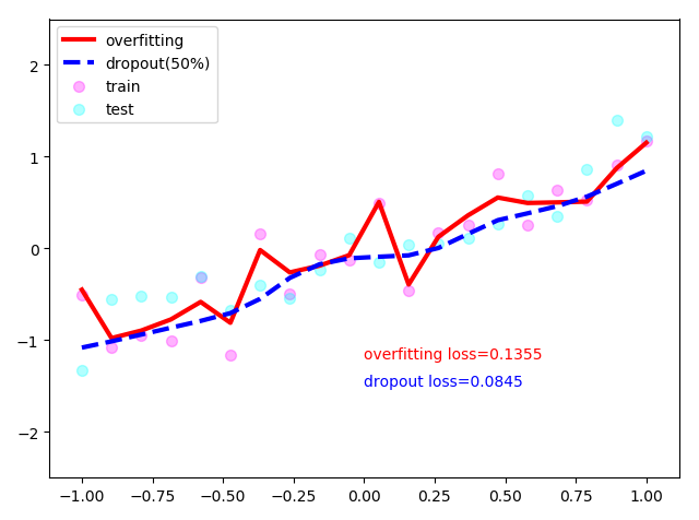
Dropout 的使用使得网络不过分依赖于少数节点，每个节点都尽可能地发挥自己的作用，他们最终对输入的微小变化不那么敏感。最后，你会得到一个更健壮的网络，它能更好地泛化。