R语言学习 - 线图绘制

线图是反映趋势变化的一种方式，其输入数据一般也是一个矩阵。

单线图

假设有这么一个矩阵，第一列为转录起始位点及其上下游5 kb的区域，第二列为H3K27ac修饰在这些区域的丰度，想绘制一张线图展示。

profile="Pos;H3K27ac
-5000;8.7
-4000;8.4
-3000;8.3
-2000;7.2
-1000;3.6
0;3.6
1000;7.1
2000;8.2
3000;8.4
4000;8.5
5000;8.5"

读入数据

profile_text <- read.table(text=profile, header=T, row.names=1, quote="",sep=";")

# 在melt时保留位置信息
# melt格式是ggplot2画图最喜欢的格式
# 好好体会下这个格式，虽然多占用了不少空间，但是确实很方便
# 这里可以用 `xvariable`，也可以是其它字符串，但需要保证后面与这里的一致
# 因为这一列是要在X轴显示，所以起名为`xvariable`。
profile_text$xvariable = rownames(profile_text)
library(ggplot2)
library(reshape2)
data_m <- melt(profile_text, id.vars=c("xvariable"))
data_m
   xvariable variable value
1      -5000  H3K27ac   8.7
2      -4000  H3K27ac   8.4
3      -3000  H3K27ac   8.3
4      -2000  H3K27ac   7.2
5      -1000  H3K27ac   3.6
6          0  H3K27ac   3.6
7       1000  H3K27ac   7.1
8       2000  H3K27ac   8.2
9       3000  H3K27ac   8.4
10      4000  H3K27ac   8.5
11      5000  H3K27ac   8.5

然后开始画图，与画heatmap一样。

# variable和value为矩阵melt后的两列的名字，内部变量, variable代表了点线的属性，value代表对应的值。
p <- ggplot(data_m, aes(x=xvariable, y=value), color=variable) + geom_line()
# 图会存储在当前目录的Rplots.pdf文件中，如果用Rstudio，可以不运行dev.off()
dev.off()

满心期待一个倒钟形曲线，结果出错了。仔细看，出来一段提示

geom_path: Each group consists of only one observation. 

Do you need to adjust the group aesthetic?

原来默认ggplot2把每个点都视作了一个分组，什么都没画出来。而data_m中的数据都来源于一个分组H3K27ac，分组的名字为variable，修改下脚本，看看效果。

p <- ggplot(data_m, aes(x=xvariable, y=value, color=variable, group=variable)) + geom_line() + theme(legend.position=c(0.1,0.9))
p

图出来了，一条线，看一眼没问题；再仔细看，不对了，怎么还不是倒钟形，原来横坐标错位了。

检查下数据格式

summary(data_m)
  xvariable      variable
 Length:11       H3K27ac:11
 Class :character
 Mode  :character

问题来了，xvariable虽然看上去像数字，但存储的实际是字符串 (因为是作为行名字读取的)，需要转换为数字。

data_m$xvariable <- as.numeric(data_m$xvariable)

#再检验下
is.numeric(data_m$xvariable)
[1] TRUE

好了，继续画图。

# 注意断行时，加号在行尾，不能放在行首
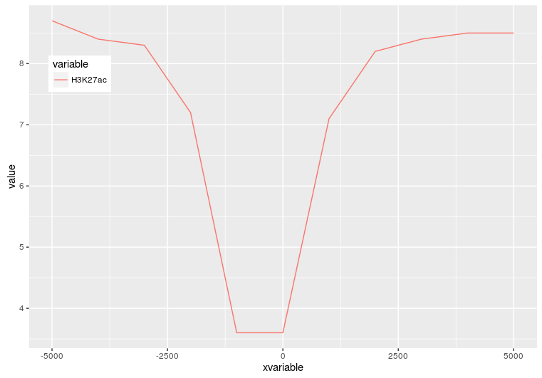
p <- ggplot(data_m, aes(x=xvariable, y=value,color=variable,group=variable)) +
     geom_line() + theme(legend.position=c(0.1,0.8))
p

图终于出来了，调了下legend的位置，看上去有点意思了

有点难看，如果平滑下，会不会好一些，stat_smooth可以对绘制的线进行局部拟合。在不影响变化趋势的情况下，可以使用 (但慎用)。

p <- ggplot(data_m, aes(x=xvariable, y=value,color=variable,group=variable)) +
     geom_line() + stat_smooth(method="auto", se=FALSE) +
     theme(legend.position=c(0.1,0.8))
p

从图中看，趋势还是一致的，线条更优美了。另外一个方式是增加区间的数量，线也会好些，而且更真实。

stat_smooth和geom_line各绘制了一条线，只保留一条就好。

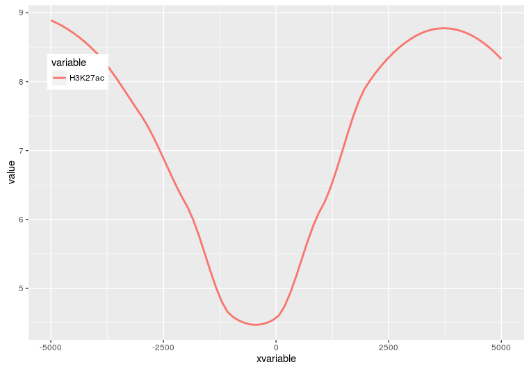
p <- ggplot(data_m, aes(x=xvariable, y=value,color=variable,group=variable)) +
     stat_smooth(method="auto", se=FALSE) + theme(legend.position=c(0.1,0.8))
p

好了，终于完成了单条线图的绘制

多线图

那么再来一个多线图的例子吧，只要给之前的数据矩阵多加几列就好了。

profile = "Pos;h3k27ac;ctcf;enhancer;h3k4me3;polII
-5000;8.7;10.7;11.7;10;8.3
-4000;8.4;10.8;11.8;9.8;7.8
-3000;8.3;10.5;12.2;9.4;7
-2000;7.2;10.9;12.7;8.4;4.8
-1000;3.6;8.5;12.8;4.8;1.3
0;3.6;8.5;13.4;5.2;1.5
1000;7.1;10.9;12.4;8.1;4.9
2000;8.2;10.7;12.4;9.5;7.7
3000;8.4;10.4;12;9.8;7.9
4000;8.5;10.6;11.7;9.7;8.2
5000;8.5;10.6;11.7;10;8.2"

profile_text <- read.table(text=profile, header=T, row.names=1, quote="",sep=";")

profile_text$xvariable = rownames(profile_text)
data_m <- melt(profile_text, id.vars=c("xvariable"))
data_m$xvariable <- as.numeric(data_m$xvariable)

# 这里group=variable，而不是group=1 (如果上面你用的是1的话)
# variable和value为矩阵melt后的两列的名字，内部变量, variable代表了点线的属性，value代表对应的值。
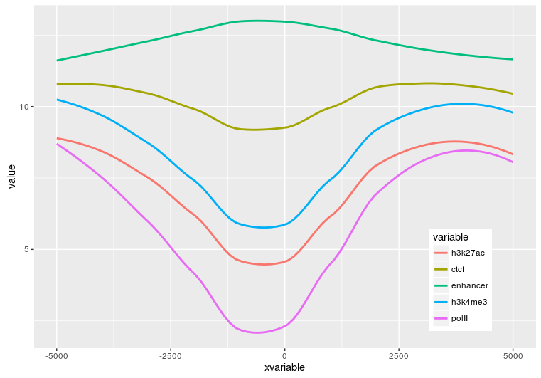
p <- ggplot(data_m, aes(x=xvariable, y=value,color=variable,group=variable)) + stat_smooth(method="auto", se=FALSE) + theme(legend.position=c(0.85,0.2))
p

横轴文本线图

如果横轴是文本，又该怎么调整顺序呢？还记得之前热图旁的行或列的顺序调整吗？重新设置变量的factor水平就可以控制其顺序。

profile = "Pos;h3k27ac;ctcf;enhancer;h3k4me3;polII
-5000;8.7;10.7;11.7;10;8.3
-4000;8.4;10.8;11.8;9.8;7.8
-3000;8.3;10.5;12.2;9.4;7
-2000;7.2;10.9;12.7;8.4;4.8
-1000;3.6;8.5;12.8;4.8;1.3
0;3.6;8.5;13.4;5.2;1.5
1000;7.1;10.9;12.4;8.1;4.9
2000;8.2;10.7;12.4;9.5;7.7
3000;8.4;10.4;12;9.8;7.9
4000;8.5;10.6;11.7;9.7;8.2
5000;8.5;10.6;11.7;10;8.2"

profile_text <- read.table(text=profile, header=T, row.names=1, quote="",sep=";")

profile_text_rownames <- row.names(profile_text)

profile_text$xvariable = rownames(profile_text)
data_m <- melt(profile_text, id.vars=c("xvariable"))

# 就是这一句，会经常用到
data_m$xvariable <- factor(data_m$xvariable, levels=profile_text_rownames, ordered=T)

# geom_line设置线的粗细和透明度
p <- ggplot(data_m, aes(x=xvariable, y=value,color=variable,group=variable)) + geom_line(size=1, alpha=0.9) + theme(legend.position=c(0.85,0.2)) + theme(axis.text.x=element_text(angle=45,hjust=1, vjust=1))

# stat_smooth
#p <- ggplot(data_m, aes(x=xvariable, y=value,color=variable,group=variable)) + stat_smooth(method="auto", se=FALSE) + theme(legend.position=c(0.85,0.2)) + theme(axis.text.x=element_text(angle=45,hjust=1, vjust=1))
p

比较下位置信息做为数字(前面的线图)和位置信息横轴的差别。当为数值时，ggplot2会选择合适的几个刻度做标记，当为文本时，会全部标记。另外文本横轴，smooth效果不明显 

到此完成了线图的基本绘制，虽然还可以，但还有不少需要提高的地方，比如在线图上加一条或几条垂线、加个水平线、修改X轴的标记(比如0换为TSS)、设置每条线的颜色等。